f-statistic

Goal. Test whether performance changes across four conditions measured on the same participants.

Design & Experiment

• Within-subjects factor: Condition with 4 levels (C1, C2, C3, C4).
• s = 8 participants measured in k = 4 conditions ⇒ total observations \(N = s \times k = 32\).
• Example context: the same students take four weekly quizzes after different study activities.

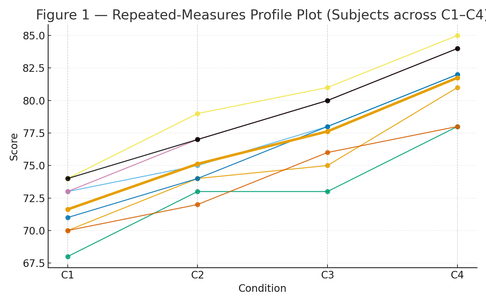
Figure 1: Profile plot (each subject as a line across the four conditions).

Data

Scores (rows = participants S1–S8; columns = conditions C1–C4):

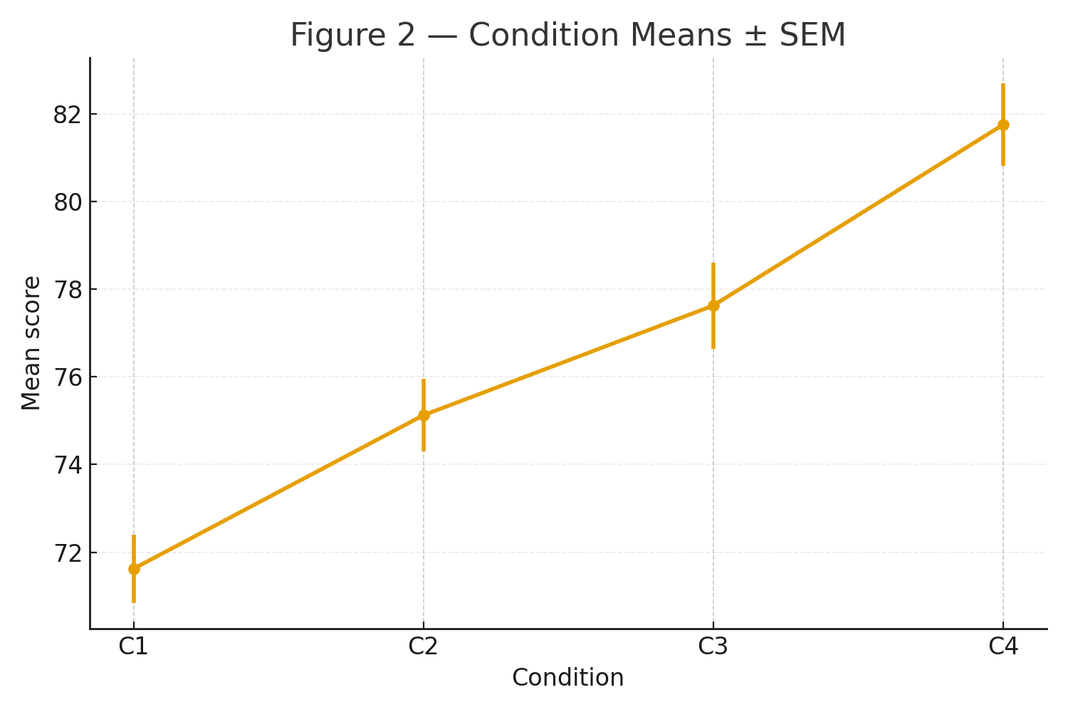
Figure 2: Means ± SEM for C1–C4 (bar/line).

Step 1 — Condition Means (and sample variances)

\[ \begin{aligned} \bar X_{\mathrm{C1}} &= 573/8 = 71.625, \quad & s^2_{\mathrm{C1}} &= 4.8393 \\ \bar X_{\mathrm{C2}} &= 601/8 = 75.125, \quad & s^2_{\mathrm{C2}} &= 5.5536 \\ \bar X_{\mathrm{C3}} &= 621/8 = 77.625, \quad & s^2_{\mathrm{C3}} &= 7.6964 \\ \bar X_{\mathrm{C4}} &= 654/8 = 81.750, \quad & s^2_{\mathrm{C4}} &= 7.0714 \end{aligned} \]

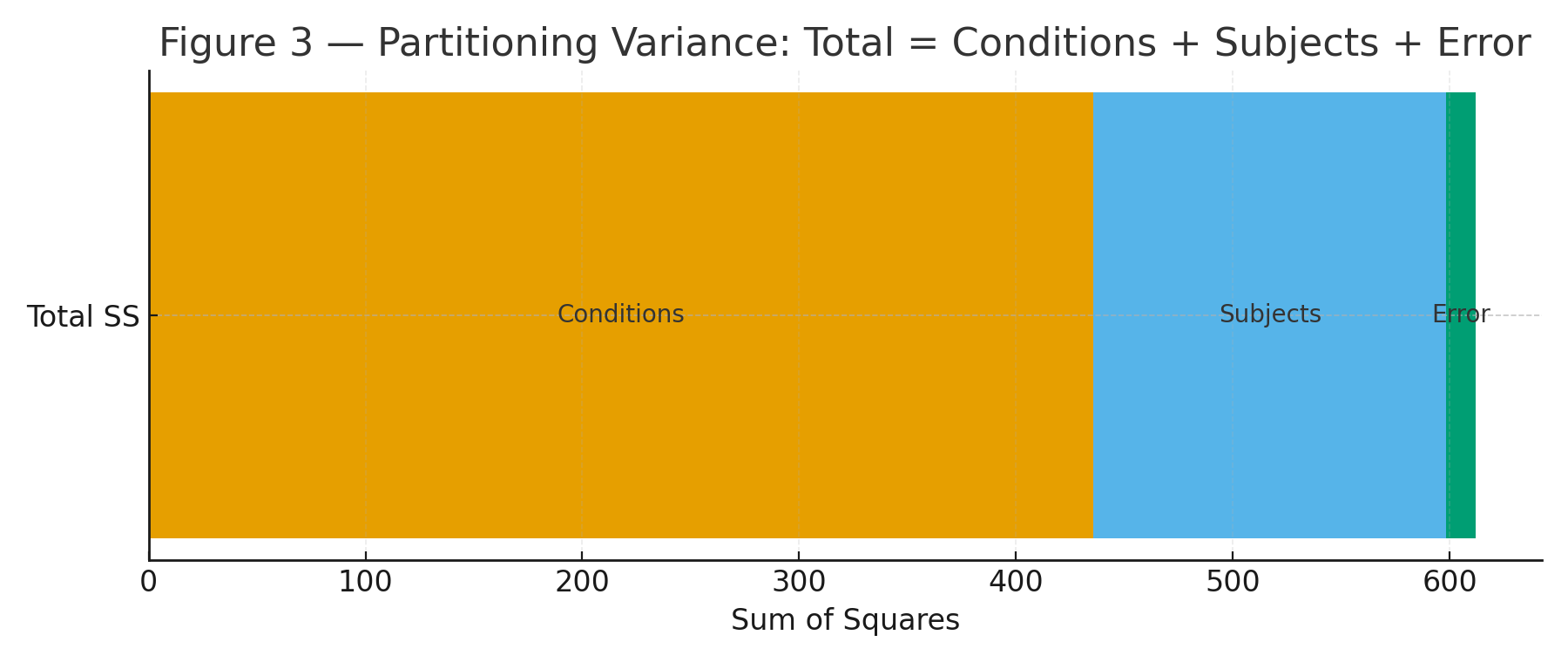
Step 2 — Sums of Squares

Notation: \(s=8\) subjects, \(k=4\) conditions, grand mean \( \bar X = 76.53125\).

2A. Total

\[ SS_{\text{total}}=\sum_{i=1}^{s}\sum_{j=1}^{k}\bigl(X_{ij}-\bar X\bigr)^2 =\mathbf{611.96875}. \]

2B. Conditions (Treatment)

\[ SS_{\text{cond}}= s \sum_{j=1}^{k}\bigl(\bar X_{\cdot j}-\bar X\bigr)^2 = 8 \left[(71.625-76.53125)^2 + (75.125-76.53125)^2 + (77.625-76.53125)^2 + (81.75-76.53125)^2\right] =\mathbf{435.84375}. \]

2C. Subjects

\[ SS_{\text{subj}}= k \sum_{i=1}^{s}\bigl(\bar X_{i\cdot}-\bar X\bigr)^2 = 4 \sum_{i=1}^{8}\bigl(\bar X_{i\cdot}-76.53125\bigr)^2 =\mathbf{162.71875}. \]

2D. Error (Residual)

\[ SS_{\text{error}}= SS_{\text{total}} - SS_{\text{cond}} - SS_{\text{subj}} = 611.96875 - 435.84375 - 162.71875 =\mathbf{13.40625}. \]

Figure 3: Partitioning variance diagram (Total → Conditions + Subjects + Error).

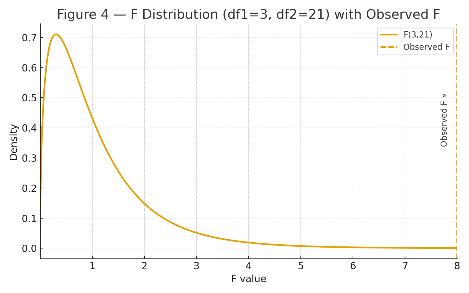
Step 3 — Degrees of Freedom & Mean Squares

\[ \begin{aligned} df_{\text{cond}} &= k-1 = 3, \\ df_{\text{subj}} &= s-1 = 7, \\ df_{\text{error}} &= (s-1)(k-1) = 7\times3 = 21, \\ df_{\text{total}} &= sk-1 = 31. \end{aligned} \]

\[ MS_{\text{cond}} = \frac{SS_{\text{cond}}}{df_{\text{cond}}} =\frac{435.84375}{3}=\mathbf{145.28125},\qquad MS_{\text{error}} = \frac{SS_{\text{error}}}{df_{\text{error}}} =\frac{13.40625}{21}=\mathbf{0.6383928571}. \]

Step 4 — Test Statistic & p-value

\[ F = \frac{MS_{\text{cond}}}{MS_{\text{error}}} = \frac{145.28125}{0.6383928571} =\mathbf{227.5734}. \] With \(df_1=3\) and \(df_2=21\), this is extremely large. The right-tail p-value is effectively \(p \lt 10^{-12}\) (i.e., \(p \ll .001\)).

Figure 4: F distribution with observed F marked and right-tail region shaded.

Repeated-Measures ANOVA Summary Table

Interpretation

Mean performance increases steadily from C1 → C4, and the repeated-measures ANOVA shows a highly significant effect of Condition, \(F(3,21)=227.57,\, p\ll .001\). Follow-ups (e.g., paired t-tests with Bonferroni/Holm) can localize which pairs of conditions differ.

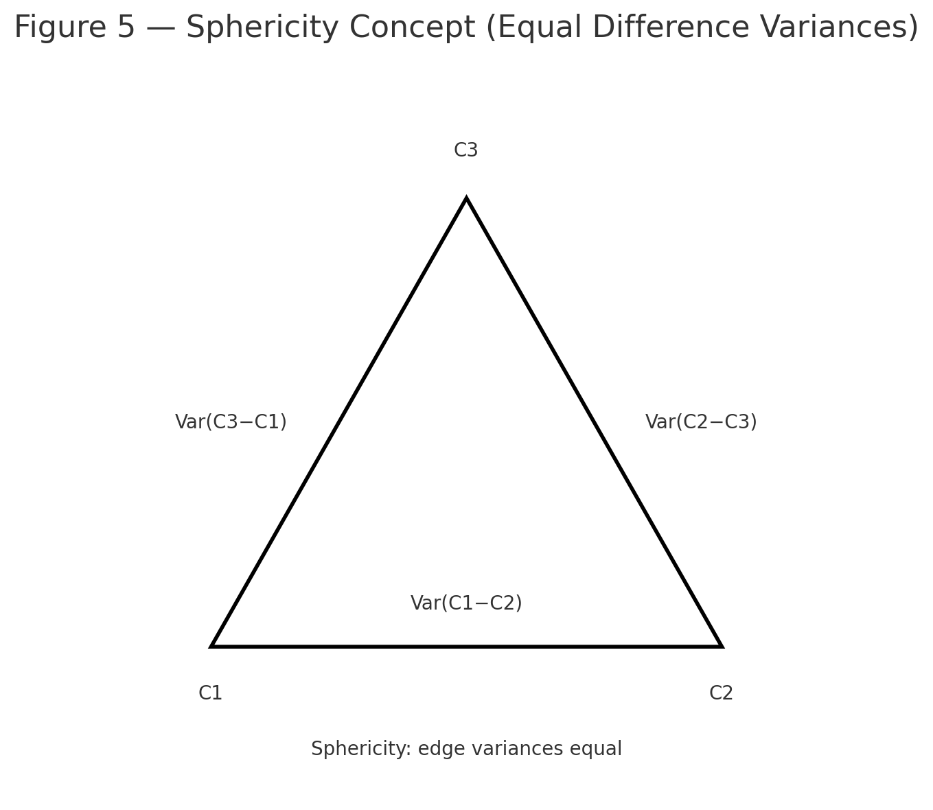
Assumptions (checklist)

• Sphericity (equal variances of the differences between condition pairs). If violated, apply Greenhouse–Geisser or Huynh–Feldt correction to \(df\).
• Approximately normal scores within each condition.
• No carryover/fatigue effects that confound order (counterbalancing helps).

Figure 5: Sphericity concept sketch (pairwise difference variances).

Practice self-test quiz

In the space below, please find practice problems and self-test quizzes. For full access, please signup free.

Goal. Test the effects of Method (Lecture vs. Online) and Time (Early vs. Late) on exam scores, and whether there is an interaction between Method and Time.

Design & Experiment

• Factor A (Method): Lecture vs. Online
• Factor B (Time): Early vs. Late
• Balanced design: \(n=5\) per cell ⇒ total \(N=20\).

Students are randomly assigned to one of four cells (Method × Time). After a short module, all students take the same 100-point exam.

Figure 1: 2 × 2 layout (Method × Time).

Data

Scores by cell (five students per cell):

Within each cell the sample variance is 4 (SD = 2), so the within-cell sum of squares is \((n-1)s^2 = 4\times4 = 16\) per cell.

Figure 2: Means with SEM by Time, separate lines for Method.

Figure 3: Interaction plot (Lecture rises sharply; Online nearly flat).

Step 1 — Marginal Means and Grand Mean

Cell means: \[ \bar X_{\text{Lecture,Early}}=70,\; \bar X_{\text{Lecture,Late}}=78,\; \bar X_{\text{Online,Early}}=72,\; \bar X_{\text{Online,Late}}=73. \] Marginal means: \[ \bar X_{\text{Lecture}}=\frac{70+78}{2}=74,\quad \bar X_{\text{Online}}=\frac{72+73}{2}=72.5; \qquad \bar X_{\text{Early}}=\frac{70+72}{2}=71,\quad \bar X_{\text{Late}}=\frac{78+73}{2}=75.5. \] Grand mean: \[ \bar X=\frac{70+78+72+73}{4}=73.25. \]

Step 2 — Sums of Squares (Between)

Balanced design formulas (with \(n\) per cell, \(a=b=2\)):

• \(SS_A = nb \sum_a(\bar X_{a\cdot}-\bar X)^2\), here \(nb=10\).
• \(SS_B = na \sum_b(\bar X_{\cdot b}-\bar X)^2\), here \(na=10\).
• \(SS_{AB} = n \sum_{a,b}\big(\bar X_{ab}-\bar X_{a\cdot}-\bar X_{\cdot b}+\bar X\big)^2\), here \(n=5\).

Compute each term:

Factor A (Method): \[ \begin{aligned} SS_A &= 10\Big[(74-73.25)^2 + (72.5-73.25)^2\Big]\\ &= 10\big[0.75^2 + (-0.75)^2\big] = 10(0.5625+0.5625)=\mathbf{11.25}. \end{aligned} \]

Factor B (Time): \[ \begin{aligned} SS_B &= 10\Big[(71-73.25)^2 + (75.5-73.25)^2\Big]\\ &= 10\big[(-2.25)^2 + (2.25)^2\big] = 10(5.0625+5.0625)=\mathbf{101.25}. \end{aligned} \]

Interaction \(A\times B\): For each cell compute \(d_{ab}=\bar X_{ab}-\bar X_{a\cdot}-\bar X_{\cdot b}+\bar X\). Here each \(d_{ab}=\pm1.75\) so \(d_{ab}^2=3.0625\) and there are four cells: \[ SS_{AB}=5\times(4\times3.0625)=\mathbf{61.25}. \]

Step 3 — Within-Group (Error) and Total SS

Within each cell, \((n-1)s^2=16\). With 4 cells: \[ SS_{\text{within}}=\mathbf{64.00}. \]

Total: \[ SS_{\text{total}}=SS_A+SS_B+SS_{AB}+SS_{\text{within}} =11.25+101.25+61.25+64.00=\mathbf{238.75}. \]

Step 4 — Degrees of Freedom & Mean Squares

\[ \begin{aligned} &df_A=a-1=1,\quad df_B=b-1=1,\quad df_{AB}=(a-1)(b-1)=1,\\ &df_{\text{within}}=N-ab=20-4=\mathbf{16},\quad df_{\text{total}}=N-1=19. \end{aligned} \] \[ MS_A=\frac{11.25}{1}=11.25,\quad MS_B=\frac{101.25}{1}=101.25,\quad MS_{AB}=\frac{61.25}{1}=61.25,\quad MS_{\text{within}}=\frac{64.00}{16}=\mathbf{4.00}. \]

Step 5 — F Tests & p-values

\[ F_A=\frac{MS_A}{MS_{\text{within}}}=\frac{11.25}{4}= \mathbf{2.8125},\qquad F_B=\frac{MS_B}{MS_{\text{within}}}=\frac{101.25}{4}= \mathbf{25.3125},\qquad F_{AB}=\frac{MS_{AB}}{MS_{\text{within}}}=\frac{61.25}{4}= \mathbf{15.3125}. \] With \(df_1=1\), \(df_2=16\): \[ p_A \approx 0.11\;(\text{n.s.}),\quad p_B < 0.001,\quad p_{AB} \approx 0.001. \]

ANOVA Summary Table

Interpretation

Main effect of Time (B) is significant: Late > Early on average. Main effect of Method (A) is not significant at conventional levels. The interaction (A × B) is significant: Lecture improves markedly from Early→Late, while Online changes little—non-parallel lines in the interaction plot.

Figure 4: Interaction plot highlighting non-parallel lines.

Assumptions (checklist)

• Independence of observations within and across cells.
• Approximately normal scores within each cell.
• Homogeneity of variances across cells (here, each cell variance ≈ 4).

Practice self-test quiz

In the space below, please find practice problems and self-test quizzes. For full access, please signup free.

A mixed design combines a between-subjects factor (different groups of participants) with a within-subjects factor (the same participants measured repeatedly).
It is also called a split-plot design.

This design is common in psychology, education, and medicine.
Example: groups of patients (between factor) measured at different time points (within factor).

Structure of the Design

• Between-subjects factor: separate groups of participants (e.g., Drug vs. Placebo).
• Within-subjects factor: repeated measures on each participant (e.g., Week 1, Week 2, Week 3).
• Interaction: tests whether the effect of the within factor depends on the between factor.

Degrees of Freedom

For a design with:

• $$a$$ levels of the between-subjects factor
• $$b$$ levels of the within-subjects factor
• $$n$$ subjects in total
• Between: $$df_{\text{between}} = a - 1$$
• Subjects (within groups): $$df_{\text{subjects}} = N - a$$
• Within: $$df_{\text{within}} = b - 1$$
• Interaction: $$df_{A \times B} = (a-1)(b-1)$$
• Error terms depend on design partitioning.

Example

Two groups of students (Drug, Placebo) are tested across three weeks.

• Between factor (Group): Drug vs. Placebo
• Within factor (Time): Weeks 1–3
• Interaction: Drug improves over time, Placebo stays flat

Symbolic Formula

$$F = \frac{MS_{\text{effect}}}{MS_{\text{error}}}$$

Where $$\text{effect}$$ may be between, within, or interaction, depending on the hypothesis.

Definition

• Mixed (split-plot) ANOVA: combines a between factor (different groups) and a within factor (repeated measures).
• Use: tests real-world designs where groups are compared across time or conditions.

Visuals

Figure L9.1 — Mixed ANOVA Layout. Two groups (Drug, Placebo) × three repeated measures (Weeks 1–3).

Figure L9.2 — Mixed ANOVA Interaction Plot. Drug group line rises sharply; Placebo line flat.

Figure L9.3 — ANOVA Summary Table for mixed design.

Why This Matters

Mixed designs are realistic and powerful.
They reflect how experiments are often run: groups compared across time.
This design unites the logic of between- and within-subjects testing.

Practice self-test quiz

In the space below, please find practice problems and self-test quizzes. For full access, please signup free.

In a repeated-measures design, the same participants are tested under multiple conditions.
This reduces error, because each person serves as their own control.
It is more powerful than a one-way ANOVA with independent groups.

Structure of the Design

• Rows (subjects): variation due to individual differences
• Columns (conditions): variation due to treatments
• Error: leftover variability after accounting for rows and columns

Degrees of Freedom

• $$df_{\text{rows}} = n - 1$$
• $$df_{\text{columns}} = k - 1$$
• $$df_{\text{error}} = (n - 1)(k - 1)$$

Where:

• $$n$$ = number of subjects
• $$k$$ = number of conditions

Example

Five students are tested under three conditions:

• Means increase steadily across conditions.
• ANOVA will partition the variance into Rows, Columns (treatments), and Error.

Symbolic Formula

$$F = \frac{MS_{\text{columns}}}{MS_{\text{error}}}$$

Formula in words:
$$F = \frac{\text{mean square for conditions}}{\text{mean square for error}}$$

Definition

• Repeated-measures ANOVA: compares means of the same group measured under different conditions.
• Advantage: controls for subject differences, increases statistical power.

Visuals

Figure L8.1 — Repeated-Measures Profile Plot. Each subject shown as a line across conditions.

Figure L8.2 — ANOVA Summary Table for repeated measures. Rows | Columns | Error.

Why This Matters

Repeated-measures designs are common in psychology, neuroscience, and medicine.
They allow researchers to detect changes over time or across treatments with fewer subjects and greater sensitivity.

Practice self-test quiz

In the space below, please find practice problems and self-test quizzes. For full access, please signup free.