degrees-of-freedom

Goal. Test the effects of Method (Lecture vs. Online) and Time (Early vs. Late) on exam scores, and whether there is an interaction between Method and Time.

Design & Experiment

• Factor A (Method): Lecture vs. Online
• Factor B (Time): Early vs. Late
• Balanced design: \(n=5\) per cell ⇒ total \(N=20\).

Students are randomly assigned to one of four cells (Method × Time). After a short module, all students take the same 100-point exam.

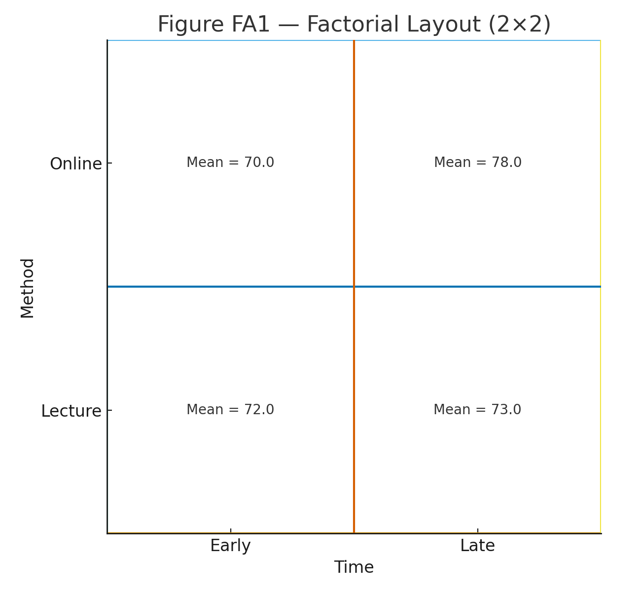
Figure 1: 2 × 2 layout (Method × Time).

Data

Scores by cell (five students per cell):

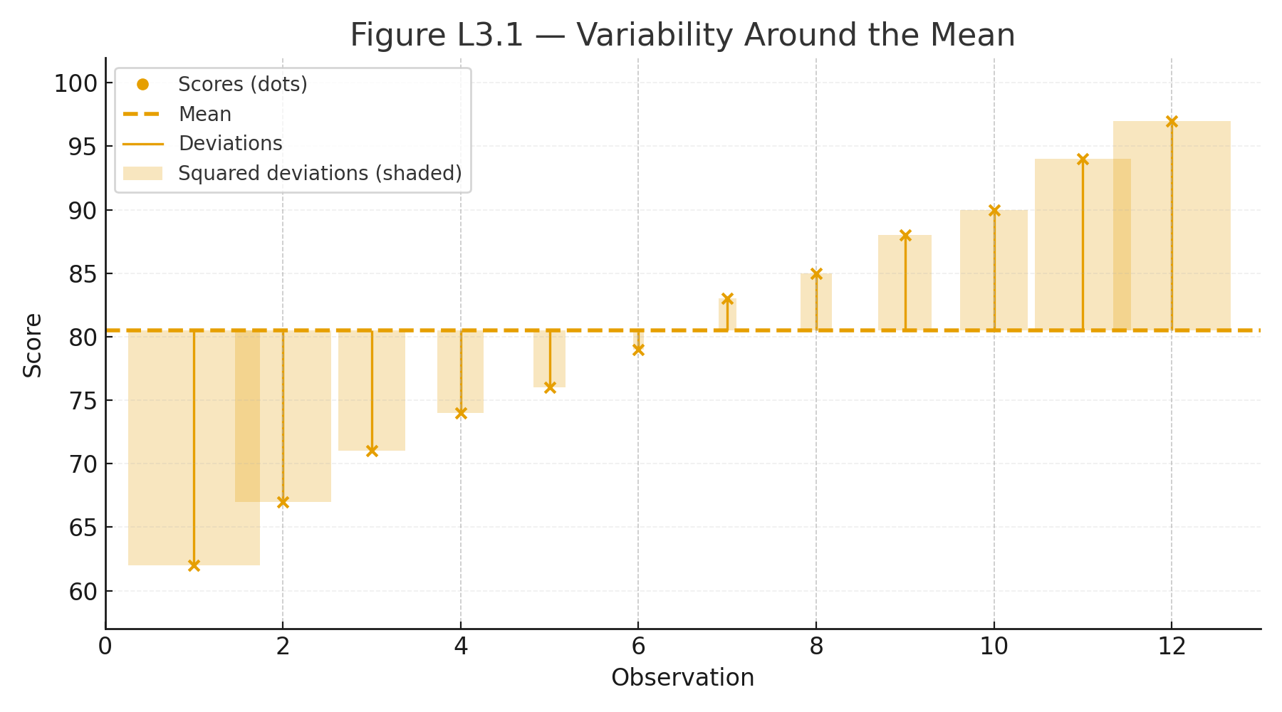
Within each cell the sample variance is 4 (SD = 2), so the within-cell sum of squares is \((n-1)s^2 = 4\times4 = 16\) per cell.

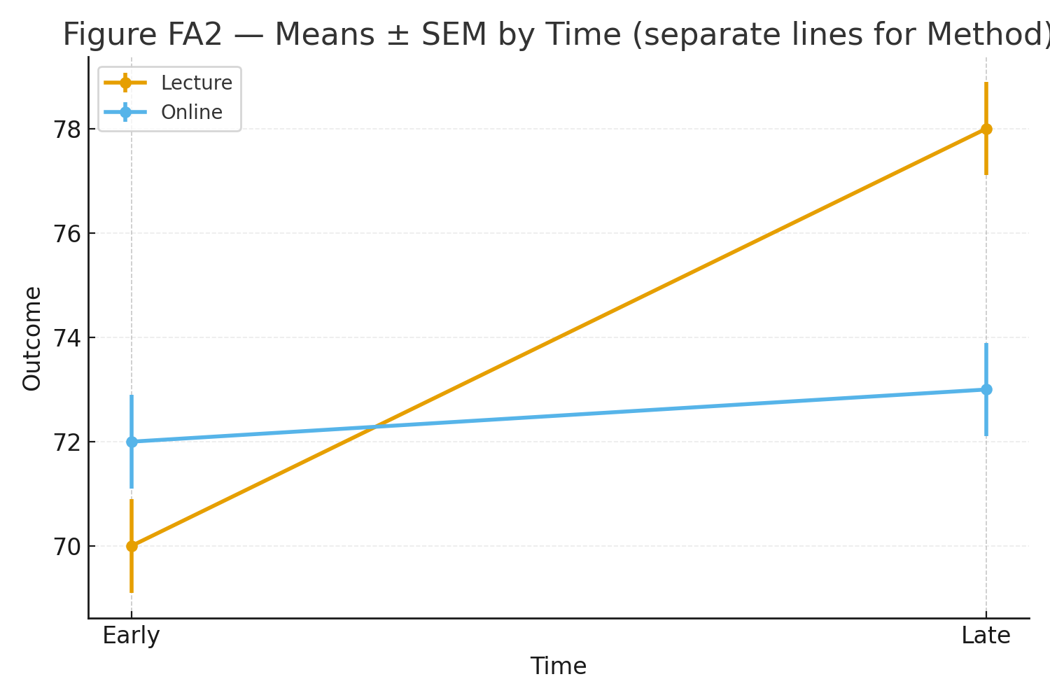
Figure 2: Means with SEM by Time, separate lines for Method.

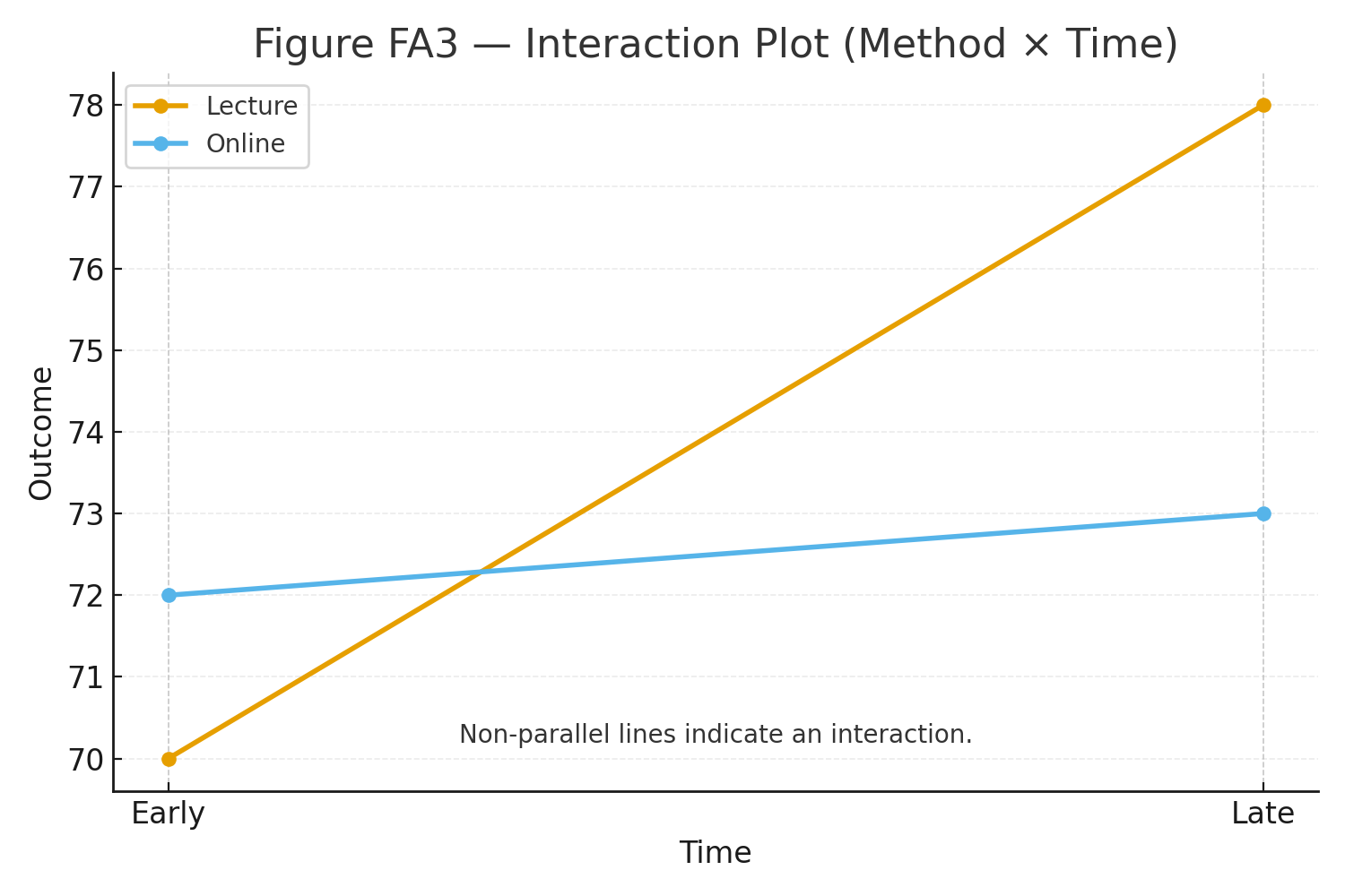
Figure 3: Interaction plot (Lecture rises sharply; Online nearly flat).

Step 1 — Marginal Means and Grand Mean

Cell means: \[ \bar X_{\text{Lecture,Early}}=70,\; \bar X_{\text{Lecture,Late}}=78,\; \bar X_{\text{Online,Early}}=72,\; \bar X_{\text{Online,Late}}=73. \] Marginal means: \[ \bar X_{\text{Lecture}}=\frac{70+78}{2}=74,\quad \bar X_{\text{Online}}=\frac{72+73}{2}=72.5; \qquad \bar X_{\text{Early}}=\frac{70+72}{2}=71,\quad \bar X_{\text{Late}}=\frac{78+73}{2}=75.5. \] Grand mean: \[ \bar X=\frac{70+78+72+73}{4}=73.25. \]

Step 2 — Sums of Squares (Between)

Balanced design formulas (with \(n\) per cell, \(a=b=2\)):

• \(SS_A = nb \sum_a(\bar X_{a\cdot}-\bar X)^2\), here \(nb=10\).
• \(SS_B = na \sum_b(\bar X_{\cdot b}-\bar X)^2\), here \(na=10\).
• \(SS_{AB} = n \sum_{a,b}\big(\bar X_{ab}-\bar X_{a\cdot}-\bar X_{\cdot b}+\bar X\big)^2\), here \(n=5\).

Compute each term:

Factor A (Method): \[ \begin{aligned} SS_A &= 10\Big[(74-73.25)^2 + (72.5-73.25)^2\Big]\\ &= 10\big[0.75^2 + (-0.75)^2\big] = 10(0.5625+0.5625)=\mathbf{11.25}. \end{aligned} \]

Factor B (Time): \[ \begin{aligned} SS_B &= 10\Big[(71-73.25)^2 + (75.5-73.25)^2\Big]\\ &= 10\big[(-2.25)^2 + (2.25)^2\big] = 10(5.0625+5.0625)=\mathbf{101.25}. \end{aligned} \]

Interaction \(A\times B\): For each cell compute \(d_{ab}=\bar X_{ab}-\bar X_{a\cdot}-\bar X_{\cdot b}+\bar X\). Here each \(d_{ab}=\pm1.75\) so \(d_{ab}^2=3.0625\) and there are four cells: \[ SS_{AB}=5\times(4\times3.0625)=\mathbf{61.25}. \]

Step 3 — Within-Group (Error) and Total SS

Within each cell, \((n-1)s^2=16\). With 4 cells: \[ SS_{\text{within}}=\mathbf{64.00}. \]

Total: \[ SS_{\text{total}}=SS_A+SS_B+SS_{AB}+SS_{\text{within}} =11.25+101.25+61.25+64.00=\mathbf{238.75}. \]

Step 4 — Degrees of Freedom & Mean Squares

\[ \begin{aligned} &df_A=a-1=1,\quad df_B=b-1=1,\quad df_{AB}=(a-1)(b-1)=1,\\ &df_{\text{within}}=N-ab=20-4=\mathbf{16},\quad df_{\text{total}}=N-1=19. \end{aligned} \] \[ MS_A=\frac{11.25}{1}=11.25,\quad MS_B=\frac{101.25}{1}=101.25,\quad MS_{AB}=\frac{61.25}{1}=61.25,\quad MS_{\text{within}}=\frac{64.00}{16}=\mathbf{4.00}. \]

Step 5 — F Tests & p-values

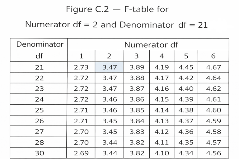
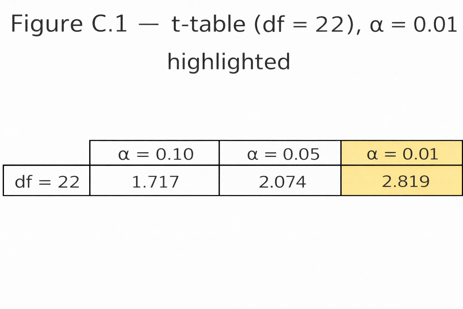
\[ F_A=\frac{MS_A}{MS_{\text{within}}}=\frac{11.25}{4}= \mathbf{2.8125},\qquad F_B=\frac{MS_B}{MS_{\text{within}}}=\frac{101.25}{4}= \mathbf{25.3125},\qquad F_{AB}=\frac{MS_{AB}}{MS_{\text{within}}}=\frac{61.25}{4}= \mathbf{15.3125}. \] With \(df_1=1\), \(df_2=16\): \[ p_A \approx 0.11\;(\text{n.s.}),\quad p_B < 0.001,\quad p_{AB} \approx 0.001. \]

ANOVA Summary Table

Interpretation

Main effect of Time (B) is significant: Late > Early on average. Main effect of Method (A) is not significant at conventional levels. The interaction (A × B) is significant: Lecture improves markedly from Early→Late, while Online changes little—non-parallel lines in the interaction plot.

Figure 4: Interaction plot highlighting non-parallel lines.

Assumptions (checklist)

• Independence of observations within and across cells.
• Approximately normal scores within each cell.
• Homogeneity of variances across cells (here, each cell variance ≈ 4).

Practice self-test quiz

In the space below, please find practice problems and self-test quizzes. For full access, please signup free.

Tables give the critical values we compare our test statistic against.
They depend on:

• The significance level (α, often 0.05)
• The degrees of freedom (df)

t-table

• Rows = degrees of freedom (df)
• Columns = significance level (α)

Example:

• Independent-samples t-test with n₁ = 12, n₂ = 12
• df = 12 + 12 – 2 = 22
• At α = 0.05 (two-tailed) → critical t ≈ 2.07
• If $$|t| \geq 2.07$$ → significant

F-table

• Needs two df values:
  • df between (numerator)
  • df within (denominator)

Example:

• One-way ANOVA, 3 groups, N = 24
• df between = k – 1 = 2
• df within = N – k = 21
• At α = 0.05 → critical F ≈ 3.47
• If computed F ≥ 3.47 → significant

Student Tips

• Always compute df correctly.
• Use tables if no software is available.
• Most calculators or apps today give exact p-values — faster than tables.

📱 QR: Interactive critical value calculator (t and F tables online)

Visuals

Figure C.1 — Snippet of a t-table row (df = 22, α = 0.05 highlighted).
Figure C.2 — F-table grid with numerator df = 2, denominator df = 21 marked.

Practice self-test quiz

In the space below, please find practice problems and self-test quizzes. For full access, please signup free.

A quick reference to the symbols used in this book.

Practice self-test quiz

In the space below, please find practice problems and self-test quizzes. For full access, please signup free.

Every statistical test requires degrees of freedom (df).
Degrees of freedom tell us how many independent pieces of information are available once totals or means are fixed.
They determine which row of the t-table or F-table we use.

General rule:

$$df = \text{number of observations} - \text{number of constraints}$$

t-tests

• One-sample t-test:
  $$df = n - 1$$
• Independent-samples t-test:
  $$df = n_1 + n_2 - 2$$
• Paired-samples t-test:
  $$df = n - 1$$

One-way ANOVA

• Between groups:
  $$df_{\text{between}} = k - 1$$
• Within groups:
  $$df_{\text{within}} = N - k$$
• Total:
  $$df_{\text{total}} = N - 1$$

Where $$k$$ = number of groups, $$N$$ = total number of scores.

Factorial ANOVA (2 × 2 Example)

• Factor A: $$df_A = a - 1$$
• Factor B: $$df_B = b - 1$$
• Interaction: $$df_{A \times B} = (a-1)(b-1)$$
• Error: $$df_{\text{within}} = N - ab$$

Repeated-Measures ANOVA

• Rows (subjects): $$df_{\text{rows}} = n - 1$$
• Columns (conditions): $$df_{\text{columns}} = k - 1$$
• Error: $$df_{\text{error}} = (n - 1)(k - 1)$$

Where $$n$$ = number of subjects, $$k$$ = number of conditions.

Mixed (Split-Plot) ANOVA

• Between factor: $$df_{\text{between}} = a - 1$$
• Subjects within groups: $$df_{\text{subjects}} = N - a$$
• Within factor: $$df_{\text{within}} = b - 1$$
• Interaction: $$df_{A \times B} = (a-1)(b-1)$$

Chi-square

• Goodness-of-fit: $$df = k - 1$$
• Independence: $$df = (r - 1)(c - 1)$$

Where $$k$$ = number of categories, $$r$$ = rows, $$c$$ = columns.

Visuals

Variables: \( n \)=sample size, \( n_1,n_2 \)=group sizes, \( N \)=total scores, \( k \)=# of groups/conditions, \( a,b \)=levels of factors A,B, \( r,c \)=rows, columns.

Why This Matters

Degrees of freedom link sample size to critical values.
They tell us how much room for variability exists in the data.
With this quick cookbook, you can locate the right df for any test.

Practice self-test quiz

In the space below, please find practice problems and self-test quizzes. For full access, please signup free.

A mixed design combines a between-subjects factor (different groups of participants) with a within-subjects factor (the same participants measured repeatedly).
It is also called a split-plot design.

This design is common in psychology, education, and medicine.
Example: groups of patients (between factor) measured at different time points (within factor).

Structure of the Design

• Between-subjects factor: separate groups of participants (e.g., Drug vs. Placebo).
• Within-subjects factor: repeated measures on each participant (e.g., Week 1, Week 2, Week 3).
• Interaction: tests whether the effect of the within factor depends on the between factor.

Degrees of Freedom

For a design with:

• $$a$$ levels of the between-subjects factor
• $$b$$ levels of the within-subjects factor
• $$n$$ subjects in total
• Between: $$df_{\text{between}} = a - 1$$
• Subjects (within groups): $$df_{\text{subjects}} = N - a$$
• Within: $$df_{\text{within}} = b - 1$$
• Interaction: $$df_{A \times B} = (a-1)(b-1)$$
• Error terms depend on design partitioning.

Example

Two groups of students (Drug, Placebo) are tested across three weeks.

• Between factor (Group): Drug vs. Placebo
• Within factor (Time): Weeks 1–3
• Interaction: Drug improves over time, Placebo stays flat

Symbolic Formula

$$F = \frac{MS_{\text{effect}}}{MS_{\text{error}}}$$

Where $$\text{effect}$$ may be between, within, or interaction, depending on the hypothesis.

Definition

• Mixed (split-plot) ANOVA: combines a between factor (different groups) and a within factor (repeated measures).
• Use: tests real-world designs where groups are compared across time or conditions.

Visuals

Figure L9.1 — Mixed ANOVA Layout. Two groups (Drug, Placebo) × three repeated measures (Weeks 1–3).

Figure L9.2 — Mixed ANOVA Interaction Plot. Drug group line rises sharply; Placebo line flat.

Figure L9.3 — ANOVA Summary Table for mixed design.

Why This Matters

Mixed designs are realistic and powerful.
They reflect how experiments are often run: groups compared across time.
This design unites the logic of between- and within-subjects testing.

Practice self-test quiz

In the space below, please find practice problems and self-test quizzes. For full access, please signup free.

In a repeated-measures design, the same participants are tested under multiple conditions.
This reduces error, because each person serves as their own control.
It is more powerful than a one-way ANOVA with independent groups.

Structure of the Design

• Rows (subjects): variation due to individual differences
• Columns (conditions): variation due to treatments
• Error: leftover variability after accounting for rows and columns

Degrees of Freedom

• $$df_{\text{rows}} = n - 1$$
• $$df_{\text{columns}} = k - 1$$
• $$df_{\text{error}} = (n - 1)(k - 1)$$

Where:

• $$n$$ = number of subjects
• $$k$$ = number of conditions

Example

Five students are tested under three conditions:

• Means increase steadily across conditions.
• ANOVA will partition the variance into Rows, Columns (treatments), and Error.

Symbolic Formula

$$F = \frac{MS_{\text{columns}}}{MS_{\text{error}}}$$

Formula in words:
$$F = \frac{\text{mean square for conditions}}{\text{mean square for error}}$$

Definition

• Repeated-measures ANOVA: compares means of the same group measured under different conditions.
• Advantage: controls for subject differences, increases statistical power.

Visuals

Figure L8.1 — Repeated-Measures Profile Plot. Each subject shown as a line across conditions.

Figure L8.2 — ANOVA Summary Table for repeated measures. Rows | Columns | Error.

Why This Matters

Repeated-measures designs are common in psychology, neuroscience, and medicine.
They allow researchers to detect changes over time or across treatments with fewer subjects and greater sensitivity.

Practice self-test quiz

In the space below, please find practice problems and self-test quizzes. For full access, please signup free.

A factorial design includes two or more factors studied at once.
This allows us to test not only the effect of each factor separately, but also whether the factors interact.

Example: 2 × 2 Design

• Factor A: Teaching method (Lecture, Online)
• Factor B: Time of day (Morning, Afternoon)

This design has 4 groups (2 levels of A × 2 levels of B).

We can test:

1. The main effect of Factor A (method).
2. The main effect of Factor B (time).
3. The interaction between method and time.

The ANOVA Partition

For a 2 × 2 design:

• Main effect A: $$df_A = a - 1$$
• Main effect B: $$df_B = b - 1$$
• Interaction A × B: $$df_{A \times B} = (a - 1)(b - 1)$$
• Error (within): $$df_{\text{within}} = N - ab$$

Where $$a$$ = levels of Factor A, $$b$$ = levels of Factor B, $$N$$ = total number of observations.

Interaction

An interaction occurs when the effect of one factor depends on the level of the other factor.

• If lines in a plot are parallel, there is no interaction.
• If lines cross or diverge, there is an interaction.

Example

Suppose means are:

• Lecture: Morning = 70, Afternoon = 90
• Online: Morning = 80, Afternoon = 80

Here:

• Main effect of method: Online > Lecture overall
• Main effect of time: Afternoon > Morning overall
• Interaction: Lecture scores rise with time, Online scores stay flat → non-parallel lines.

Visuals

Figure L7.1 — Factorial Layout (2 × 2). A 2 × 2 grid: Method × Time.

Figure L7.2 — Interaction Plot. Lecture line slopes upward, Online line flat. Caption: “Lines not parallel = interaction.”

Figure L7.3 — ANOVA Summary Table for 2 × 2 design. Source | SS | df | MS | F | p.

Why This Matters

Factorial designs let us test more than one factor at a time.
They are efficient and powerful, and the concept of interaction is central in science.
Two-way ANOVA is the foundation for more complex designs, including repeated measures and mixed ANOVA.

Practice self-test quiz

In the space below, please find practice problems and self-test quizzes. For full access, please signup free.

The t-test compares two means. But what if we have three or more groups?
We could run multiple t-tests, but that inflates the chance of error.

The solution is the Analysis of Variance (ANOVA).
ANOVA partitions the variability into two parts: between groups and within groups.

Partitioning the Variance

Total variability = variability between groups + variability within groups.

• Between groups: differences due to the factor (treatment).
• Within groups: differences due to chance or individual variation.

Symbolic formula:
$$F = \frac{MS_{\text{between}}}{MS_{\text{within}}}$$

Formula in words:
$$F = \frac{\text{mean square between groups}}{\text{mean square within groups}}$$

Where:

• $$MS_{\text{between}} = \tfrac{SS_{\text{between}}}{df_{\text{between}}}$$
• $$MS_{\text{within}} = \tfrac{SS_{\text{within}}}{df_{\text{within}}}$$

Degrees of Freedom

• $$df_{\text{between}} = k - 1$$
• $$df_{\text{within}} = N - k$$
• $$df_{\text{total}} = N - 1$$

Where $$k$$ = number of groups, $$N$$ = total number of observations.

Example (One-way ANOVA)

Three groups of students use different study techniques:

• Group A: mean = 70
• Group B: mean = 75
• Group C: mean = 85

Suppose calculations give:

• $$SS_{\text{between}} = 300, , df_{\text{between}} = 2 \Rightarrow MS_{\text{between}} = 150$$
• $$SS_{\text{within}} = 200, , df_{\text{within}} = 12 \Rightarrow MS_{\text{within}} = 16.7$$

Then:

$$F = \frac{150}{16.7} = 9.0$$

This F value is compared to the F table at df = (2, 12).

Definition

• ANOVA: compares means across three or more groups.
• F ratio: signal-to-noise ratio (treatment effect vs. error).

Visual Placeholders

Figure L6.1 — Partitioning Variance. Total variability divided into Between vs. Within.

Figure L6.2 — One-way ANOVA Layout. Bar graph with three groups (A, B, C).

Figure L6.3 — ANOVA Summary Table. Source | SS | df | MS | F | p.

Why This Matters

ANOVA generalizes the t-test to multiple groups.
It is one of the most widely used tools in psychology, education, and medicine.
Understanding the F ratio is key: a large F means treatment differences are greater than chance variation. 

Practice self-test quiz

In the space below, please find practice problems and self-test quizzes. For full access, please signup free.

This lecture emphasizes conceptual understanding of the t-test, its logic, and how it fits into the broader structure of statistical reasoning.

The t-test is one of the most widely used statistical tools.
It compares two means and asks: Is the difference between them real, or could it be due to chance?

The t-test is closely related to the z-test.
When the population standard deviation is unknown and the sample size is small, we use t instead of z.

Types of t-Tests

• One-sample t-test: compares a sample mean to a known or hypothesized population mean.
• Independent-samples t-test: compares means from two separate groups.
• Paired-samples t-test: compares two scores from the same group (before vs. after).

Symbolic Formulas

One-sample t-test
$$t = \frac{\bar{X} - \mu_0}{s / \sqrt{n}}$$

Independent-samples t-test
$$t = \frac{\bar{X}_1 - \bar{X}_2}{\sqrt{\tfrac{s_1^2}{n_1} + \tfrac{s_2^2}{n_2}}}$$

Paired-samples t-test
$$t = \frac{\bar{D}}{s_D / \sqrt{n}}$$

Degrees of Freedom

• One-sample: $$df = n - 1$$
• Independent-samples: $$df = n_1 + n_2 - 2$$
• Paired-samples: $$df = n - 1$$

Example (Independent t-Test)

Two groups of students try different study methods:

• Group A: \(n = 10\), mean = 80, SD = 10
• Group B: \(n = 10\), mean = 90, SD = 10

$$t = \frac{80 - 90}{\sqrt{\tfrac{10^2}{10} + \tfrac{10^2}{10}}} = \frac{-10}{\sqrt{10 + 10}} = \frac{-10}{\sqrt{20}} = \frac{-10}{4.47} = -2.24$$

Degrees of freedom = 18.
Compare this t-value to the critical value in the t-table at \(df = 18\).

Example (Paired t-Test)

Students take a test before and after tutoring.
Differences (After − Before): 4, 6, 5, 3, 2.

Mean difference:
$$\bar{D} = \frac{4 + 6 + 5 + 3 + 2}{5} = 4$$

Standard deviation of differences:
$$s_D = 1.58$$

$$t = \frac{4}{1.58 / \sqrt{5}} = \frac{4}{0.71} = 5.63$$

Degrees of freedom = 4.
This large t-value indicates strong evidence of improvement.

Definition

• Independent t-test: compares two separate groups.
• Paired t-test: compares the same group measured twice.
• Degrees of freedom (df): number of independent pieces of information.

Visuals

Figure L5.1 — Independent t-Test. Bar graph of two groups (A and B) with means and SEM error bars.

Figure L5.2 — Paired t-Test. Line plot showing before vs. after scores for each student.

Figure L5.3 — t vs. z Distribution. Overlay of the normal (z) curve and t curves with df = 5 and 20.

Why This Matters

The t-test is the workhorse of statistics.
It forms the foundation for many other methods (ANOVA, regression, mixed models).
Understanding t means understanding how we compare signal (mean difference) to noise (variability).

Practice self-test quiz

In the space below, please find practice problems and self-test quizzes. For full access, please signup free.

The mean tells us the “typical” score. But how tightly do scores cluster around the mean? Do they spread widely, or are they close together?

To answer, we measure variability. Two key measures are the variance and the standard deviation.

Variance

Variance is the average squared distance of scores from the mean.

Symbolic formula:
$$s^2 = \frac{\sum (X - \bar{X})^2}{n - 1}$$

Formula in words:
$$\text{Variance} = \frac{\text{sum of squared deviations from the mean}}{\text{number of scores} - 1}$$

Where:

• $$s^2$$ = variance
• $$X$$ = each score
• $$\bar{X}$$ = mean
• $$n$$ = number of scores

Standard Deviation

The standard deviation is the square root of the variance. It puts variability back into the same units as the data.

Symbolic formula:
$$s = \sqrt{\frac{\sum (X - \bar{X})^2}{n - 1}}$$

Formula in words:
$$\text{Standard deviation} = \sqrt{\frac{\text{sum of squared deviations from the mean}}{\text{number of scores} - 1}}$$

Example

Data: 6, 8, 10

• Mean = 8
• Deviations: –2, 0, 2
• Squared deviations: 4, 0, 4
• Sum = 8

Variance:
$$s^2 = \frac{8}{3-1} = 4$$

Standard deviation:
$$s = \sqrt{4} = 2$$

So, on average, scores are 2 units away from the mean.

Definition

• Variance: average squared distance from the mean.
• Standard Deviation: square root of variance; typical distance from the mean.

Visuals

Figure L3.1 — Variability Around the Mean. Dot plot of scores with the mean marked, vertical lines for deviations, and shaded boxes for squared deviations.

Why This Matters

Two sets of scores can have the same mean but very different spreads.
Variance and standard deviation give us the language to describe spread, and they are the building blocks for t-tests, ANOVA, and all inferential statistics.

Practice self-test quiz

In the space below, please find practice problems and self-test quizzes. For full access, please signup free.