

Lecture 2 — The Goddess Normal Curve
The normal curve (bell curve) is one of the most important concepts in statistics.
It is elegant, symmetrical, and central to probability and inference.
It appears whenever many small, independent factors combine: height, exam scores, measurement errors.
Properties of the Normal Curve
- Symmetrical around the mean
- One peak (unimodal)
- Mean = Median = Mode
- Total area under the curve = 1 (100%)
Formula for the Normal Distribution
Symbolic formula:
$$f(x) = \frac{1}{\sigma \sqrt{2\pi}} e^{-\frac{(x - \mu)^2}{2\sigma^2}}$$
Formula in words:
$$\text{Probability density} = \frac{1}{\text{standard deviation} \times \sqrt{2\pi}} \times e^{-\frac{(\text{score} - \text{mean})^2}{2 \times (\text{standard deviation})^2}}$$
Where:
- $$\mu$$ = mean
- $$\sigma$$ = standard deviation
- $$x$$ = a score
Standardization (z-scores)
Symbolic formula:
$$z = \frac{x - \mu}{\sigma}$$
Formula in words:
$$z = \frac{\text{score} - \text{mean}}{\text{standard deviation}}$$
A z-score tells us how many standard deviations a score is above or below the mean.
Key Percentages
Under the normal curve:
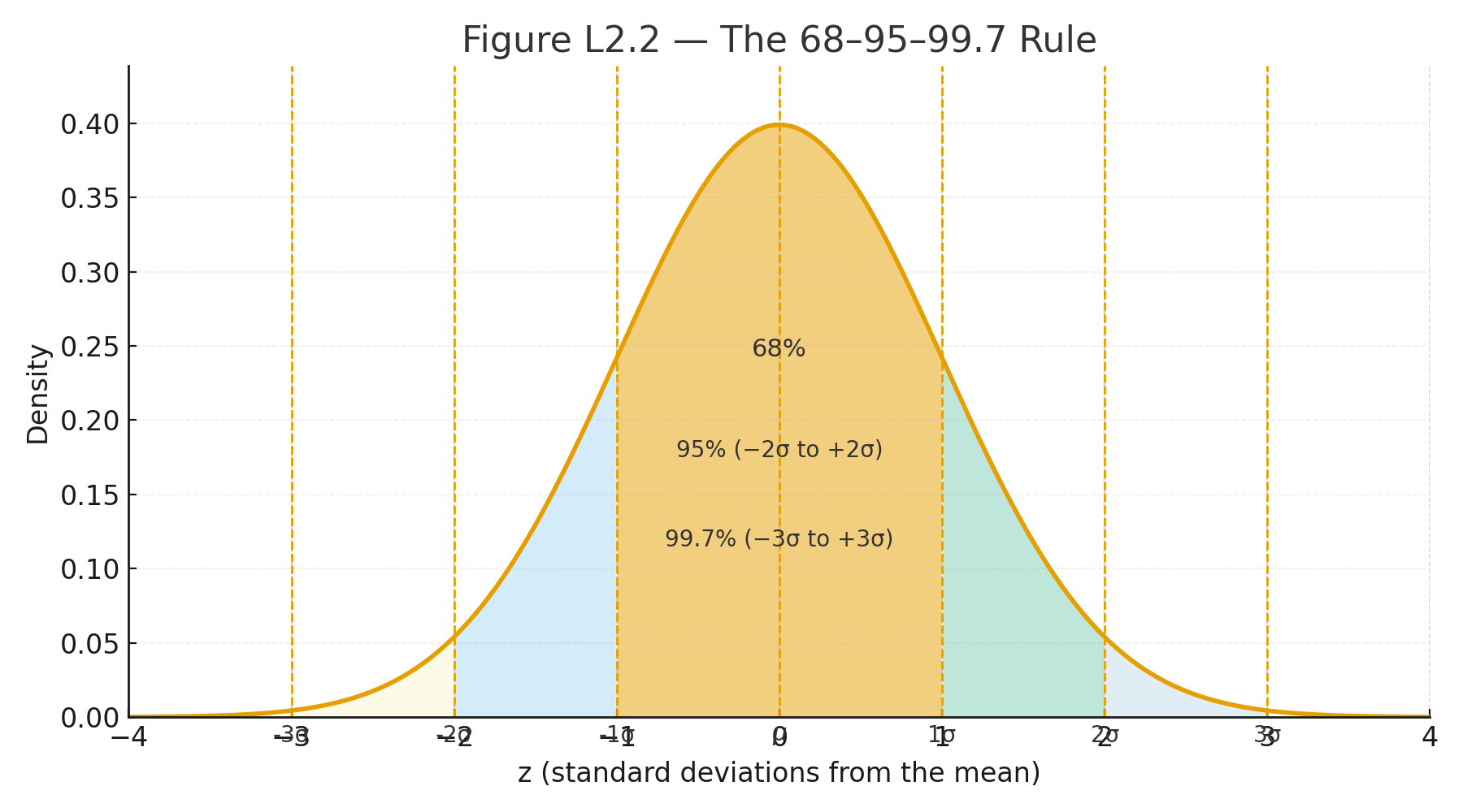
- About 68% of scores are within 1 standard deviation of the mean
- About 95% are within 2 standard deviations
- About 99.7% are within 3 standard deviations
This is called the 68–95–99.7 rule.
Drama Box — “The Goddess Normal Curve”
Imagine a temple where a perfect curve stands tall — balanced and symmetrical.
- At the center is the mean, the balance point.
- Half of the people (data) stand on each side.
- As you move further away, fewer remain.
- The Goddess teaches fairness: most scores are near the center, extreme scores are rare.
This image helps students remember the normal curve not as a dry formula, but as a principle of balance and probability.
Visuals
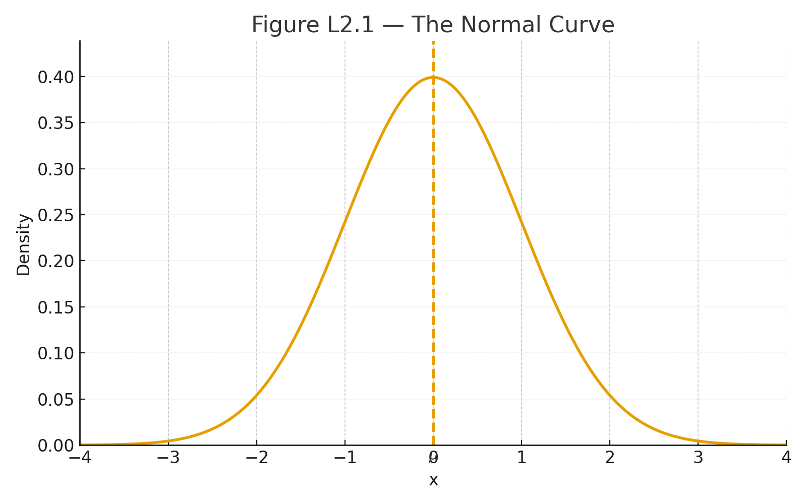
Figure L2.1 — The Normal Curve. Bell-shaped curve centered at the mean (μ).
Figure L2.2 — The 68–95–99.7 Rule. Normal curve with shaded regions ±1σ, ±2σ, ±3σ.
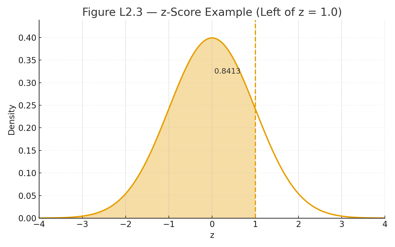
Figure L2.3 — z-score Example. Normal curve with shaded area to the left of z = 1.0, labeled 0.8413.
Why This Matters
The normal curve is the foundation of inferential statistics.
- It allows us to calculate probabilities.
- It underlies t-tests, ANOVAs, and confidence intervals.
- It lets us compare scores across different tests and scales.
Practice self-test quiz
In the space below, please find practice problems and self-test quizzes. For full access, please signup free.