standard-deviation

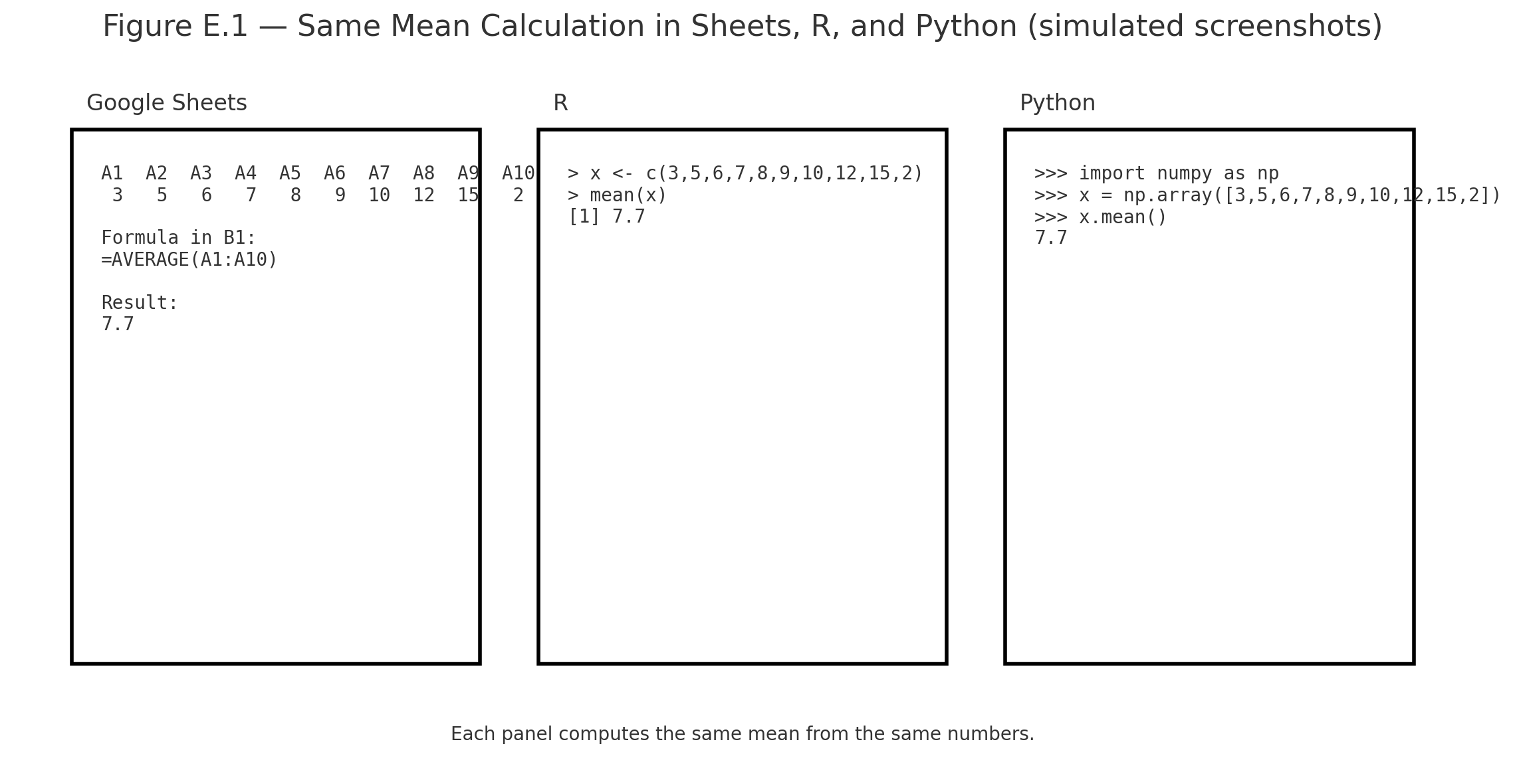
Mean (average)
Sum of all scores divided by number of scores.
Example: (6 + 8 + 10) / 3 = 8.

Median
Middle score when data are ordered.
Example: For [5, 7, 8], median = 7.

Mode
Most frequent score.
Example: For [2, 3, 3, 5], mode = 3.

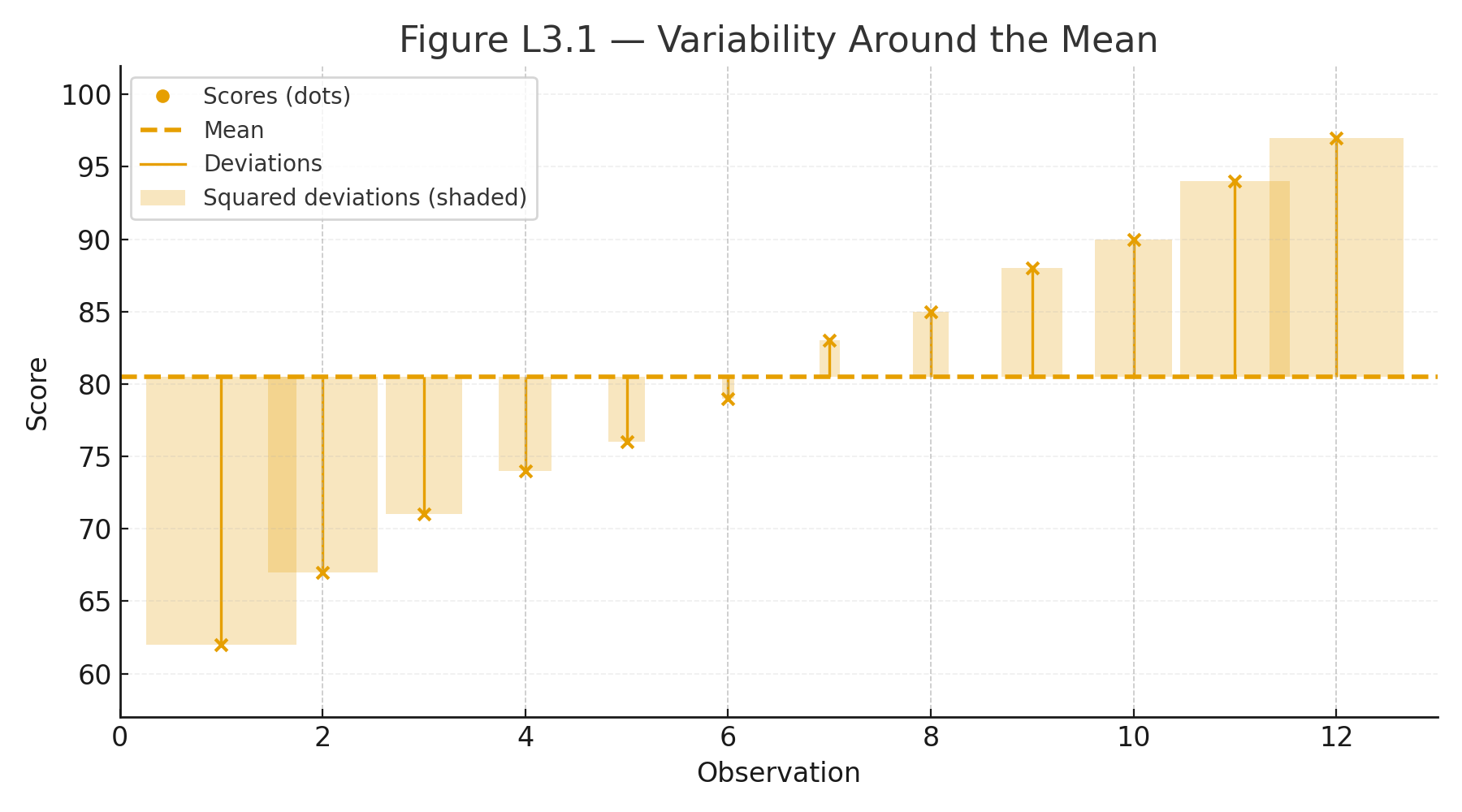
Variance (s²)
Average squared deviation from the mean.

Standard Deviation (s)
Square root of variance. Spread of scores around the mean.

Standard Error of the Mean (SEM)
How much sample means vary.
Formula: $$SEM = \frac{s}{\sqrt{n}}$$

t-test
Compares two means.

ANOVA (F-test)
Compares three or more means.

Post Hoc Test
Used after ANOVA to find which groups differ.

Correlation (r)
Strength and direction of a linear relationship. Range: –1 to +1.

Regression
Equation that predicts Y from X.
Example: $$\hat{Y} = a + bX$$

Chi-square (χ²)
Test for categorical data (counts).

Degrees of Freedom (df)
Independent pieces of information in a test.

p-value
Probability of getting the observed result (or more extreme) if the null hypothesis is true.

📱 QR: Interactive glossary (search symbols, formulas, definitions)

Practice self-test quiz

In the space below, please find practice problems and self-test quizzes. For full access, please signup free.

Learning statistics is not about memorizing formulas — it’s about thinking with data.
Here are some strategies to make it easier.

1. Read Formulas in Two Ways

• Symbolic: $$\bar{X} = \frac{\Sigma X}{n}$$
• Words: “Mean = sum of scores / number of scores”

2. Practice by Hand First

• Work out a mean or variance with a small dataset.
• Then check with calculator/Excel.
• This builds intuition and confidence.

3. Draw Pictures

• Normal curve with shaded area
• Bar charts for group means
• Scatterplots for correlation
  Visuals make ideas stick.

4. Watch Out for Common Mistakes

• Mixing up SD and SEM
• Forgetting to subtract 1 for df
• Using a one-tailed test when two-tailed is needed

5. Use Short Sessions

• 10–15 minutes of practice each day beats one long cram.
• Try one formula or test per session.

6. Check Your Understanding

• Can you explain in words what the test does?
• Example: “t-test compares two means. ANOVA compares three or more.”

📱 QR: Online flashcards + short quiz (practice key terms & formulas)

Practice self-test quiz

In the space below, please find practice problems and self-test quizzes. For full access, please signup free.

Statistics can be done with calculators, spreadsheets, or software. Here’s a quick guide.

Excel / Google Sheets

R (RStudio or RStudio Cloud)

Python (NumPy / SciPy / Pandas)

iPhone Calculator

• Rotate sideways → scientific mode
• Use √ for square root
• Parentheses matter: type numerator, then divide by denominator
• Fine for small problems, but not for full datasets

Summary

• For quick homework: iPhone calculator
• For assignments: Excel / Google Sheets
• For coding: Python (Colab) or R (RStudio Cloud)

📱 QR: Open sample data in Google Sheets (ready to practice mean, SD, t-test)

Visuals

Figure E.1 — Screenshots of the same mean calculation in Sheets, R, and Python side by side.

Practice self-test quiz

In the space below, please find practice problems and self-test quizzes. For full access, please signup free.

The z-table gives areas (probabilities) under the standard normal curve (mean $$\mu=0$$, SD $$\sigma=1$$).
Use it after you standardize a score:

Standardization (z-score):
$$z=\frac{x-\mu}{\sigma}$$
In words: $$z=\frac{\text{score} - \text{mean}}{\text{standard deviation}}$$

What the z-table shows

Most tables list the area to the left of a z value (cumulative probability).

• Left area at $$z=0$$ is 0.5000 (half the curve).
• Far left (negative big z) approaches 0; far right (positive big z) approaches 1.

Quick recipes

1) Probability below a score (left tail)
Example: $$z=1.00$$ → table gives 0.8413.
Interpretation: $$P(Z \le 1.00)=0.8413$$ (84.13% below).

2) Probability above a score (right tail)
Use complement: $$P(Z \ge z)=1-\text{left area}$$.
Example: $$z=1.00 \Rightarrow P(Z \ge 1.00)=1-0.8413=0.1587.$$

3) Probability between two scores
Subtract left areas.
Example: between $$z= -0.50$$ (left area 0.3085) and $$z=1.20$$ (0.8849):
$$P(-0.50 \le Z \le 1.20)=0.8849-0.3085=0.5764.$$

4) From a raw score to probability
Test scores: $$\mu=100, \ \sigma=15$$. What % are below 115?
Standardize: $$z=\frac{115-100}{15}=1.00 \Rightarrow 0.8413 \ (\text{84.13%}).$$

5) From probability to raw score (percentile)
What score is the 90th percentile?
Find z with left area ≈ 0.9000 → $$z \approx 1.2816$$.
Convert back: $$x=\mu+z\sigma=100+(1.2816)(15)=119.22.$$

Tips

• For negative z, use the table’s symmetry: left area at $$-z$$ equals 1 − left area at $$+z$$.
• Rounding: two decimals is common (e.g., 1.23).
• Modern tools (calculator/Sheets/Python) can give exact p-values directly.

Visuals

Figure D.1 — Normal curve with area left of z = 1.00 shaded (0.8413).
Figure D.2 — Two-z shaded band for “between” probability.

📱 QR: Online z-calculator (type z or x, get areas instantly)

Practice self-test quiz

In the space below, please find practice problems and self-test quizzes. For full access, please signup free.

A quick refresher on the math you’ll need in this book.

Order of Operations (PEMDAS)

• Parentheses → Exponents → Multiplication/Division → Addition/Subtraction
• Example:
  $$3 + 2 \times (4^2) = 3 + 2 \times 16 = 35$$

Fractions and Division

• Example:
  $$\frac{24}{6} = 4$$

Square Roots

• Example:
  $$\sqrt{9} = 3$$
• Example:
  $$\sqrt{\frac{16}{4}} = \sqrt{4} = 2$$

Summation Notation (Σ)

• Means “add them up.”
• Example:
  $$\Sigma X = 2+5+7 = 14$$
• Example:
  $$\Sigma (X-\bar{X})^2 = (2-4)^2 + (5-4)^2 + (7-4)^2 = 4+1+9 = 14$$

Exponents and Squares

• $$x^2 = x \times x$$
• Example:
  $$5^2 = 25$$

Mini Example: Variance and Standard Deviation

Data: 6, 8, 10

1. Mean:
   $$\bar{X} = \frac{6+8+10}{3} = 8$$
2. Deviations: –2, 0, +2
3. Squared deviations: 4, 0, 4
4. Variance:
   $$\frac{8}{2} = 4$$
5. Standard deviation:
   $$\sqrt{4} = 2$$

📱 QR: Algebra refresher video (scan for a quick math warm-up)

Practice self-test quiz

In the space below, please find practice problems and self-test quizzes. For full access, please signup free.

A quick reference to the symbols used in this book.

Practice self-test quiz

In the space below, please find practice problems and self-test quizzes. For full access, please signup free.

The mean tells us the “typical” score. But how tightly do scores cluster around the mean? Do they spread widely, or are they close together?

To answer, we measure variability. Two key measures are the variance and the standard deviation.

Variance

Variance is the average squared distance of scores from the mean.

Symbolic formula:
$$s^2 = \frac{\sum (X - \bar{X})^2}{n - 1}$$

Formula in words:
$$\text{Variance} = \frac{\text{sum of squared deviations from the mean}}{\text{number of scores} - 1}$$

Where:

• $$s^2$$ = variance
• $$X$$ = each score
• $$\bar{X}$$ = mean
• $$n$$ = number of scores

Standard Deviation

The standard deviation is the square root of the variance. It puts variability back into the same units as the data.

Symbolic formula:
$$s = \sqrt{\frac{\sum (X - \bar{X})^2}{n - 1}}$$

Formula in words:
$$\text{Standard deviation} = \sqrt{\frac{\text{sum of squared deviations from the mean}}{\text{number of scores} - 1}}$$

Example

Data: 6, 8, 10

• Mean = 8
• Deviations: –2, 0, 2
• Squared deviations: 4, 0, 4
• Sum = 8

Variance:
$$s^2 = \frac{8}{3-1} = 4$$

Standard deviation:
$$s = \sqrt{4} = 2$$

So, on average, scores are 2 units away from the mean.

Definition

• Variance: average squared distance from the mean.
• Standard Deviation: square root of variance; typical distance from the mean.

Visuals

Figure L3.1 — Variability Around the Mean. Dot plot of scores with the mean marked, vertical lines for deviations, and shaded boxes for squared deviations.

Why This Matters

Two sets of scores can have the same mean but very different spreads.
Variance and standard deviation give us the language to describe spread, and they are the building blocks for t-tests, ANOVA, and all inferential statistics.

Practice self-test quiz

In the space below, please find practice problems and self-test quizzes. For full access, please signup free.

The normal curve (bell curve) is one of the most important concepts in statistics.
It is elegant, symmetrical, and central to probability and inference.
It appears whenever many small, independent factors combine: height, exam scores, measurement errors.

Properties of the Normal Curve

1. Symmetrical around the mean
2. One peak (unimodal)
3. Mean = Median = Mode
4. Total area under the curve = 1 (100%)

Formula for the Normal Distribution

Symbolic formula:
$$f(x) = \frac{1}{\sigma \sqrt{2\pi}} e^{-\frac{(x - \mu)^2}{2\sigma^2}}$$

Formula in words:
$$\text{Probability density} = \frac{1}{\text{standard deviation} \times \sqrt{2\pi}} \times e^{-\frac{(\text{score} - \text{mean})^2}{2 \times (\text{standard deviation})^2}}$$

Where:

• $$\mu$$ = mean
• $$\sigma$$ = standard deviation
• $$x$$ = a score

Standardization (z-scores)

Symbolic formula:
$$z = \frac{x - \mu}{\sigma}$$

Formula in words:
$$z = \frac{\text{score} - \text{mean}}{\text{standard deviation}}$$

A z-score tells us how many standard deviations a score is above or below the mean.

Key Percentages

Under the normal curve:

• About 68% of scores are within 1 standard deviation of the mean
• About 95% are within 2 standard deviations
• About 99.7% are within 3 standard deviations

This is called the 68–95–99.7 rule.

Drama Box — “The Goddess Normal Curve”

Imagine a temple where a perfect curve stands tall — balanced and symmetrical.

• At the center is the mean, the balance point.
• Half of the people (data) stand on each side.
• As you move further away, fewer remain.
• The Goddess teaches fairness: most scores are near the center, extreme scores are rare.

This image helps students remember the normal curve not as a dry formula, but as a principle of balance and probability.

Visuals

Figure L2.1 — The Normal Curve. Bell-shaped curve centered at the mean (μ).

Figure L2.2 — The 68–95–99.7 Rule. Normal curve with shaded regions ±1σ, ±2σ, ±3σ.

Figure L2.3 — z-score Example. Normal curve with shaded area to the left of z = 1.0, labeled 0.8413.

Why This Matters

The normal curve is the foundation of inferential statistics.

• It allows us to calculate probabilities.
• It underlies t-tests, ANOVAs, and confidence intervals.
• It lets us compare scores across different tests and scales.

Practice self-test quiz

In the space below, please find practice problems and self-test quizzes. For full access, please signup free.