probability-calculation

The normal distribution is not just a shape — it is a powerful tool.
It allows us to describe data, calculate probabilities, and make decisions about means and differences.

Here are four major uses of the normal curve.

1. Describing Data

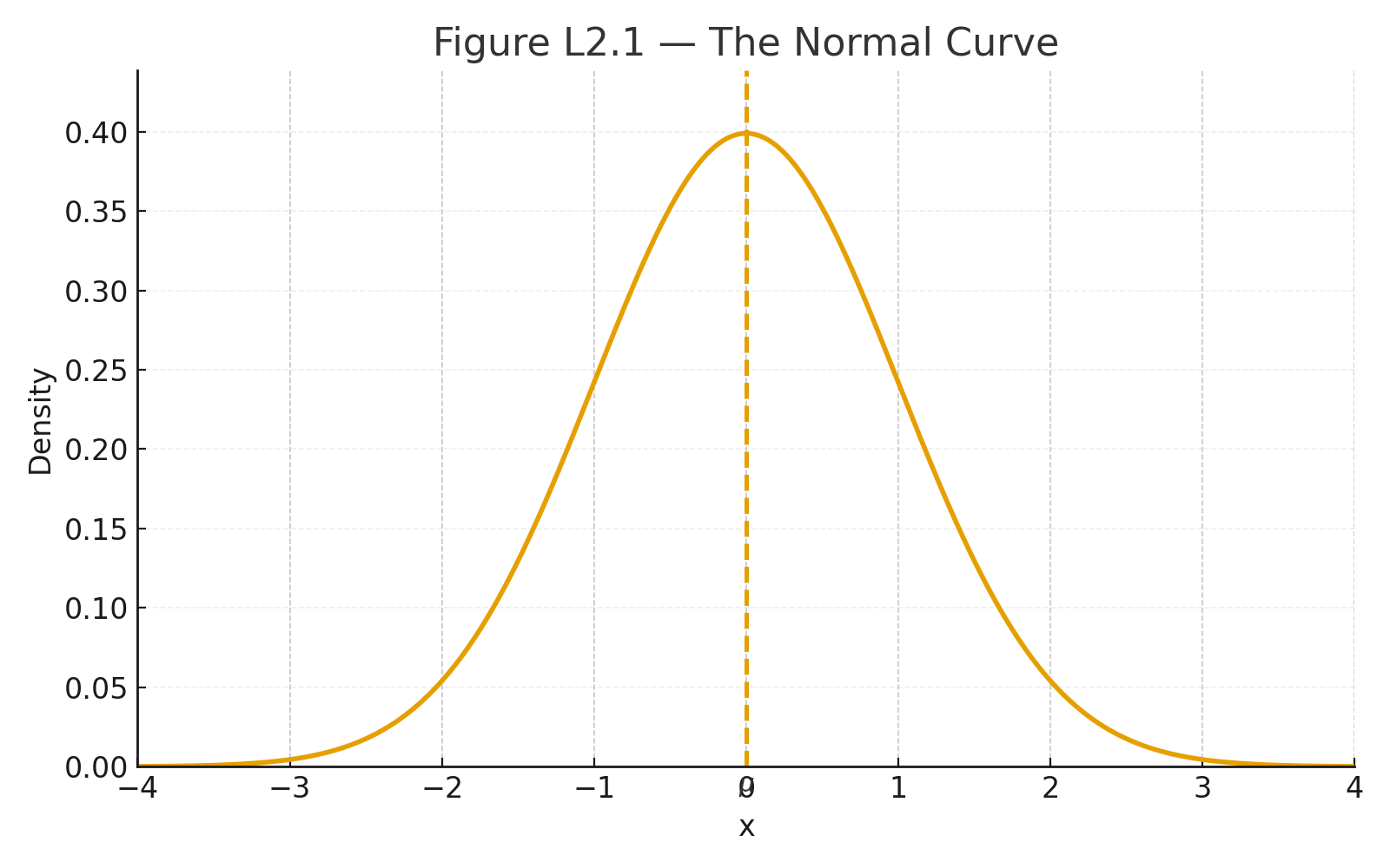
The normal curve summarizes how scores are distributed.

• Mean = center
• Standard deviation = spread

It provides a reference point: where most scores fall, and where extremes occur.

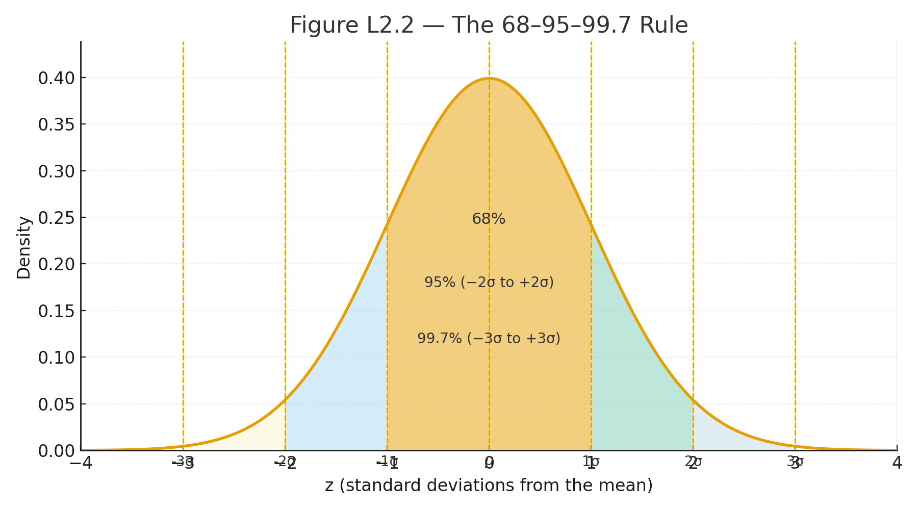
Figure L4.1 — Normal Curve with mean and ±1σ, ±2σ, ±3σ marked.

2. Probability of a Score

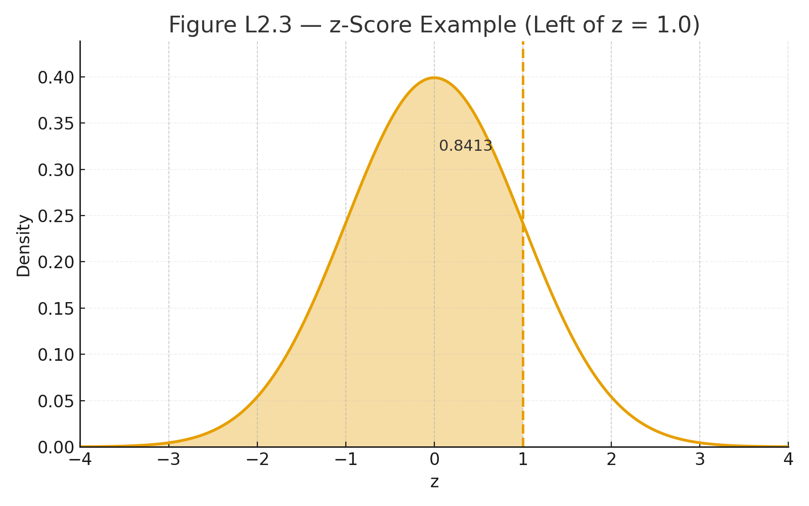
We can use the normal curve to calculate the probability of observing a score above or below a certain value.

Formula for standardization:
$$z = \frac{x - \mu}{\sigma}$$

Formula in words:
$$z = \frac{\text{score} - \text{mean}}{\text{standard deviation}}$$

The z-score tells us how many standard deviations a score is from the mean.
With the z-table, we can find the probability of that score.

Figure L4.2 — Normal curve with shaded area above z = 1.5.

3. Reliability of a Mean (SEM)

If we take many samples, the means vary. The Standard Error of the Mean (SEM) tells us how much.

Formula:
$$\mathrm{SEM} = \frac{s}{\sqrt{n}}$$

Formula in words:
$$\text{SEM} = \frac{\text{standard deviation}}{\sqrt{\text{number of scores}}}$$

Smaller SEM means the sample mean is a more reliable estimate of the population mean.

Figure L4.3 — Distribution of sample means, narrower than distribution of raw scores.

4. Reliability of a Difference

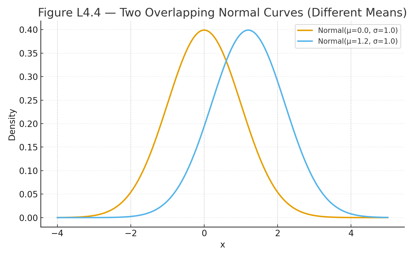
The normal distribution also underlies hypothesis testing — such as the t-test.
It allows us to compare two means and decide whether their difference is larger than expected by chance.

Figure L4.4 — Two overlapping normal curves with different means.

Why This Matters

The normal distribution is the foundation for:

• Calculating probabilities
• Estimating reliability of means
• Testing hypotheses about differences

Understanding these uses prepares us for the transition from descriptive to inferential statistics.

Practice self-test quiz

In the space below, please find practice problems and self-test quizzes. For full access, please signup free.

The normal curve (bell curve) is one of the most important concepts in statistics.
It is elegant, symmetrical, and central to probability and inference.
It appears whenever many small, independent factors combine: height, exam scores, measurement errors.

Properties of the Normal Curve

1. Symmetrical around the mean
2. One peak (unimodal)
3. Mean = Median = Mode
4. Total area under the curve = 1 (100%)

Formula for the Normal Distribution

Symbolic formula:
$$f(x) = \frac{1}{\sigma \sqrt{2\pi}} e^{-\frac{(x - \mu)^2}{2\sigma^2}}$$

Formula in words:
$$\text{Probability density} = \frac{1}{\text{standard deviation} \times \sqrt{2\pi}} \times e^{-\frac{(\text{score} - \text{mean})^2}{2 \times (\text{standard deviation})^2}}$$

Where:

• $$\mu$$ = mean
• $$\sigma$$ = standard deviation
• $$x$$ = a score

Standardization (z-scores)

Symbolic formula:
$$z = \frac{x - \mu}{\sigma}$$

Formula in words:
$$z = \frac{\text{score} - \text{mean}}{\text{standard deviation}}$$

A z-score tells us how many standard deviations a score is above or below the mean.

Key Percentages

Under the normal curve:

• About 68% of scores are within 1 standard deviation of the mean
• About 95% are within 2 standard deviations
• About 99.7% are within 3 standard deviations

This is called the 68–95–99.7 rule.

Drama Box — “The Goddess Normal Curve”

Imagine a temple where a perfect curve stands tall — balanced and symmetrical.

• At the center is the mean, the balance point.
• Half of the people (data) stand on each side.
• As you move further away, fewer remain.
• The Goddess teaches fairness: most scores are near the center, extreme scores are rare.

This image helps students remember the normal curve not as a dry formula, but as a principle of balance and probability.

Visuals

Figure L2.1 — The Normal Curve. Bell-shaped curve centered at the mean (μ).

Figure L2.2 — The 68–95–99.7 Rule. Normal curve with shaded regions ±1σ, ±2σ, ±3σ.

Figure L2.3 — z-score Example. Normal curve with shaded area to the left of z = 1.0, labeled 0.8413.

Why This Matters

The normal curve is the foundation of inferential statistics.

• It allows us to calculate probabilities.
• It underlies t-tests, ANOVAs, and confidence intervals.
• It lets us compare scores across different tests and scales.

Practice self-test quiz

In the space below, please find practice problems and self-test quizzes. For full access, please signup free.