sampling-distribution

Classical statistics uses formulas and tables.
Modern computing gives us another way: resampling and simulation.

Instead of relying only on theory, we let the computer generate thousands of samples and see what happens.

Bootstrapping

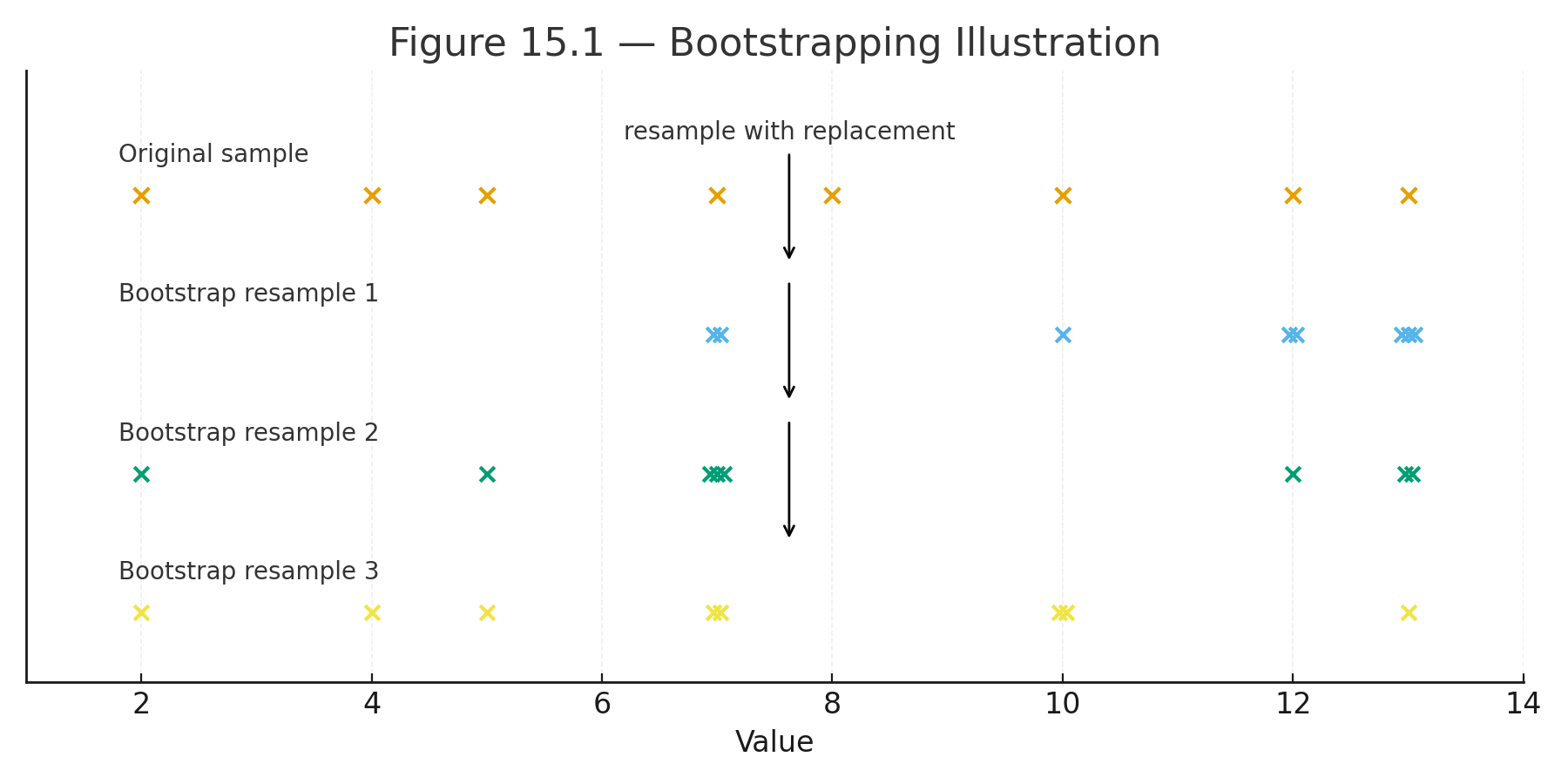
Bootstrapping means resampling with replacement from the original data.

Steps:

1. Take a sample of size $$n$$ from the data (with replacement).
2. Compute the statistic (mean, median, correlation).
3. Repeat thousands of times.
4. Use the distribution of resampled statistics to estimate confidence intervals.

Example:
Data = [5, 6, 7, 9].
Resample 1000 times, compute mean each time.
The distribution of means gives an estimate of the true mean’s variability.

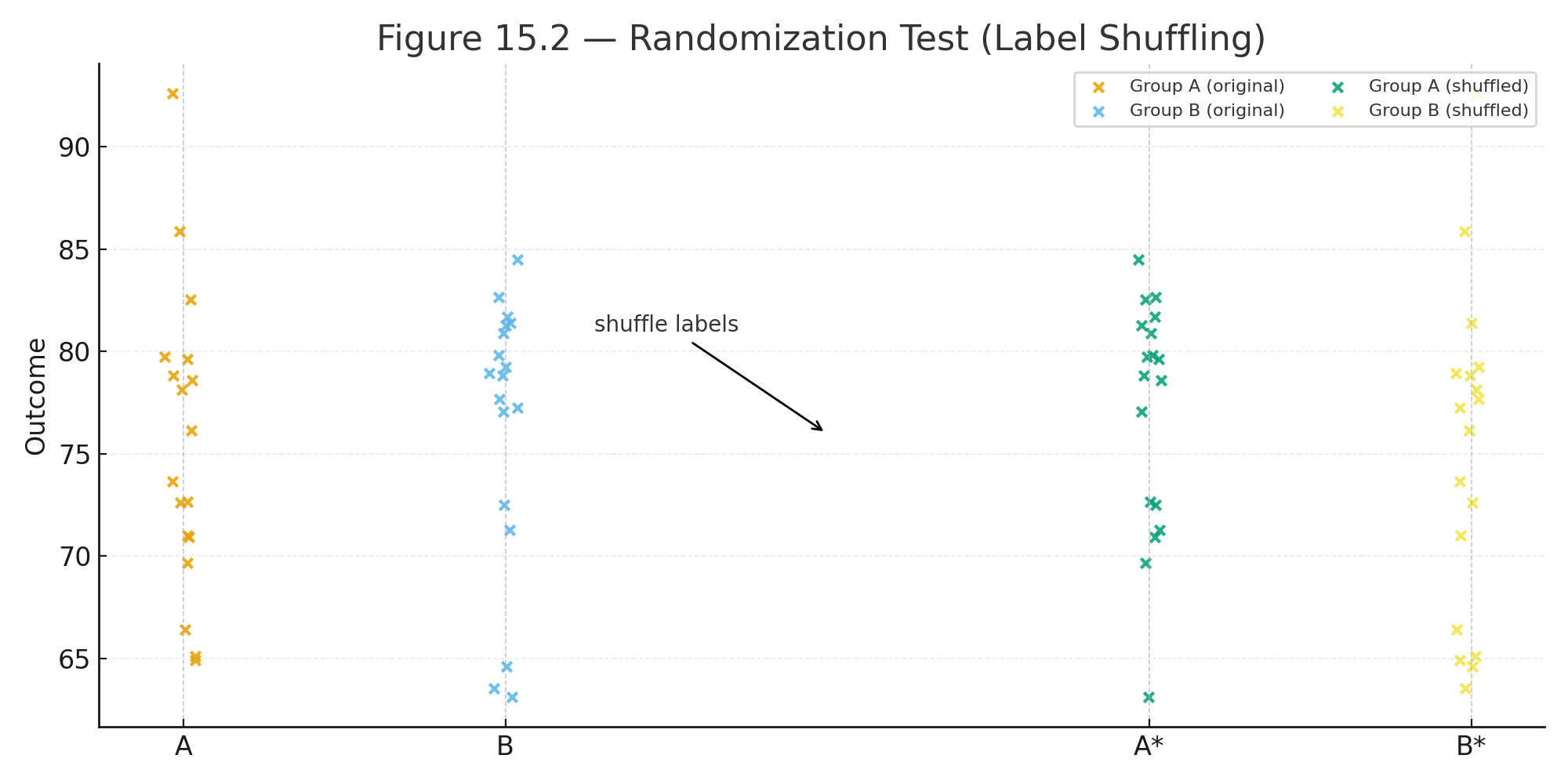
Randomization (Permutation) Tests

Used to test hypotheses by shuffling labels.

Steps:

1. Combine all data.
2. Randomly assign to groups.
3. Compute the difference in means.
4. Repeat thousands of times.
5. Compare the observed difference to this distribution.

This shows whether the observed effect could be due to chance.

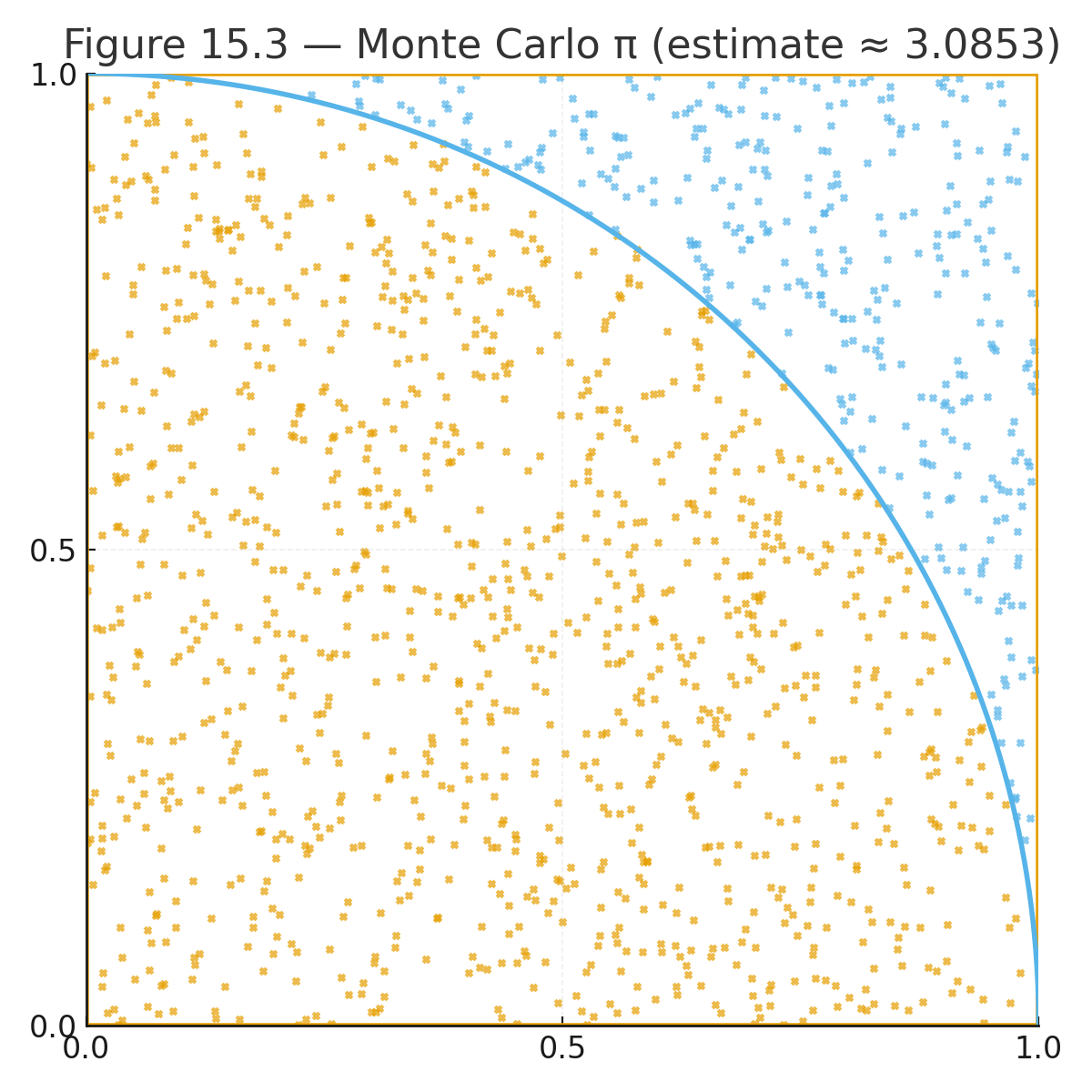
Monte Carlo Simulation

Monte Carlo methods use random numbers to model complex processes.

Example: Estimating $$\pi$$.

• Randomly throw points into a square.
• Count how many fall inside the circle quarter.
• $$\pi \approx 4 \times \tfrac{\text{inside circle}}{\text{total points}}$$.

Why Resampling Works

Resampling uses the data itself as a model of the population.
It avoids assumptions (like normality) and adapts to modern computing power.

Visuals

Figure 15.1 — Bootstrapping illustration: resampling from a small dataset with replacement.

Figure 15.2 — Randomization test: labels shuffled between groups.

Figure 15.3 — Monte Carlo: random points filling a square and a quarter circle.

Why This Matters

Resampling and simulation show students that statistics is not only about formulas.
Computers allow us to see probability in action.
This approach prepares students for data science, where simulation is as important as theory.

Practice self-test quiz

In the space below, please find practice problems and self-test quizzes. For full access, please signup free.

The normal distribution is not just a shape — it is a powerful tool.
It allows us to describe data, calculate probabilities, and make decisions about means and differences.

Here are four major uses of the normal curve.

1. Describing Data

The normal curve summarizes how scores are distributed.

• Mean = center
• Standard deviation = spread

It provides a reference point: where most scores fall, and where extremes occur.

Figure L4.1 — Normal Curve with mean and ±1σ, ±2σ, ±3σ marked.

2. Probability of a Score

We can use the normal curve to calculate the probability of observing a score above or below a certain value.

Formula for standardization:
$$z = \frac{x - \mu}{\sigma}$$

Formula in words:
$$z = \frac{\text{score} - \text{mean}}{\text{standard deviation}}$$

The z-score tells us how many standard deviations a score is from the mean.
With the z-table, we can find the probability of that score.

Figure L4.2 — Normal curve with shaded area above z = 1.5.

3. Reliability of a Mean (SEM)

If we take many samples, the means vary. The Standard Error of the Mean (SEM) tells us how much.

Formula:
$$\mathrm{SEM} = \frac{s}{\sqrt{n}}$$

Formula in words:
$$\text{SEM} = \frac{\text{standard deviation}}{\sqrt{\text{number of scores}}}$$

Smaller SEM means the sample mean is a more reliable estimate of the population mean.

Figure L4.3 — Distribution of sample means, narrower than distribution of raw scores.

4. Reliability of a Difference

The normal distribution also underlies hypothesis testing — such as the t-test.
It allows us to compare two means and decide whether their difference is larger than expected by chance.

Figure L4.4 — Two overlapping normal curves with different means.

Why This Matters

The normal distribution is the foundation for:

• Calculating probabilities
• Estimating reliability of means
• Testing hypotheses about differences

Understanding these uses prepares us for the transition from descriptive to inferential statistics.

Practice self-test quiz

In the space below, please find practice problems and self-test quizzes. For full access, please signup free.