computational-statistics

Artificial Intelligence (AI) aims to build systems that can learn, adapt, and make decisions.
One powerful tool is the neural network, inspired by the brain.

From Statistics to AI

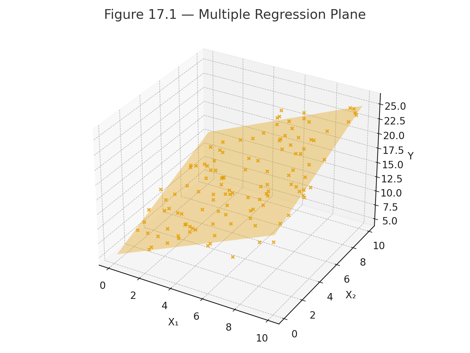
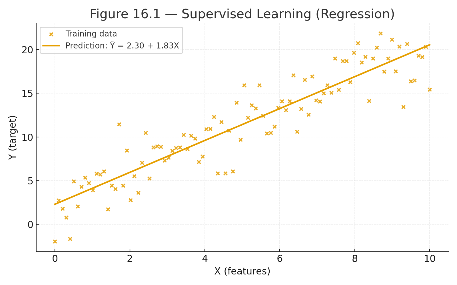
• Regression predicts Y from X
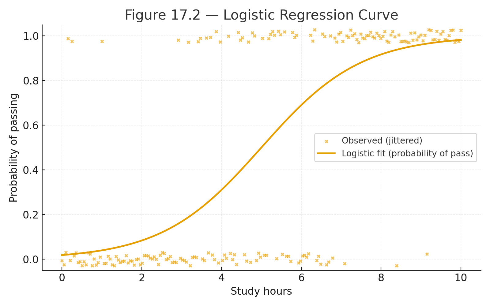
• Logistic regression predicts probability (0–1)
• Neural networks generalize this idea: many inputs, many layers, nonlinear patterns

The Structure of a Neural Network

1. Input layer — variables (X₁, X₂, …)
2. Hidden layers — units that transform the input
3. Output layer — prediction or classification

Each connection has a weight (like a slope in regression).

Formula for a Neuron

A single unit in the network:

$$z = \sum w_i X_i + b$$

$$y = f(z)$$

Where:

• $$w_i$$ = weights
• $$X_i$$ = inputs
• $$b$$ = bias (like an intercept)
• $$f(z)$$ = activation function (e.g., logistic, ReLU)

Learning in a Network

The network predicts outputs and compares them with the true answers.
The error is sent backward through the network to adjust weights.
This is called backpropagation.

Example

Predicting if a student will pass or fail based on:

• Study hours
• Attendance
• Practice problems completed

Inputs → combined with weights → logistic activation → output: probability of passing.

Visuals

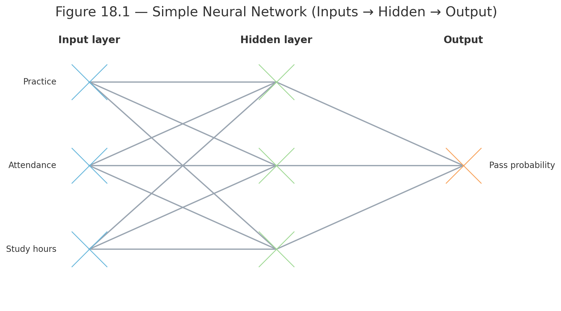
Figure 18.1 — Simple Neural Network (Inputs → Hidden → Output)

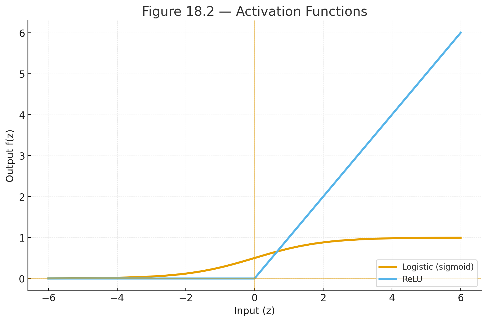
Figure 18.2 — Activation Functions

Why This Matters

• Neural networks extend regression and logistic regression.
• They allow learning from large, complex datasets (images, speech, language).
• Modern AI (translation, recognition, chatbots) is powered by these models.

Practice self-test quiz

In the space below, please find practice problems and self-test quizzes. For full access, please signup free.

Simple regression predicts Y from one X.
But in real life, outcomes often depend on several variables — or may not be linear.

This chapter introduces multiple regression and logistic regression.

Multiple Regression

Formula:

$$\hat{Y} = a + b_1X_1 + b_2X_2 + \dots + b_kX_k$$

In words:
$$\text{Predicted Y} = \text{intercept} + (b_1 \times X_1) + (b_2 \times X_2) + \dots$$

Where:

• $$X_1, X_2, \dots X_k$$ = predictors
• $$b_1, b_2, \dots b_k$$ = slopes (weights for each predictor)

Example: Predicting college GPA from:

• High school GPA ($$X_1$$)
• Study hours ($$X_2$$)

Equation:
$$\hat{Y} = 1.0 + 0.5X_1 + 0.1X_2$$

Interpretation:

• For each 1-point increase in HS GPA, college GPA rises 0.5.
• For each extra study hour, GPA rises 0.1.

Coefficient of Determination

In multiple regression, $$R^2$$ tells us the proportion of variance explained by all predictors together.

Example: $$R^2 = 0.65$$ → predictors explain 65% of the outcome’s variability.

Logistic Regression

What if the outcome is yes/no (categorical)?
Example: Will a student pass or fail?

We use logistic regression.

Formula:

$$P(Y=1) = \frac{1}{1 + e^{-(a + bX)}}$$

In words:
$$\text{Probability of success} = \frac{1}{1 + e^{-(\text{intercept} + \text{slope} \times X)}}$$

Output: probability between 0 and 1.

Example: Predicting pass/fail from study hours.

• Equation: $$P = \frac{1}{1 + e^{-( -2 + 0.5X )}}$$
• If X = 6 hours: $$P = \frac{1}{1 + e^{-1}} = 0.73$$
• About 73% chance of passing.

Visuals

Figure 17.1 — Multiple regression plane: Y predicted from two predictors.

Figure 17.2 — Logistic regression curve: probability vs. study hours.

Why This Matters

• Multiple regression = prediction with many factors
• Logistic regression = prediction when the outcome is categorical
• $$R^2$$ = strength of prediction

These methods expand the power of regression beyond a straight line, preparing for modern predictive modeling.

Practice self-test quiz

In the space below, please find practice problems and self-test quizzes. For full access, please signup free.

Machine learning is where statistics meets computers.
Instead of only writing formulas, we teach a computer to learn patterns from data.

What is Machine Learning?

Machine learning uses algorithms to improve automatically with experience.

• Supervised learning: the computer is given examples with correct answers.
• Unsupervised learning: the computer finds patterns without answers.

Supervised Learning

Goal: predict Y from X.

Examples:

• Predict exam scores from study hours
• Predict house price from size, location, and age

Steps:

1. Split data into training set and test set
2. Train the model on training data
3. Test accuracy on new (unseen) data

Formula (simple linear regression as machine learning):
$$\hat{Y} = a + bX$$

Here, the computer “learns” $$a$$ and $$b$$ from the data.

Unsupervised Learning

Goal: find hidden structure in the data.

Examples:

• Group students by study habits
• Cluster shoppers by buying patterns

Algorithms:

• k-means clustering
• Hierarchical clustering

No “correct answer” is given — the computer organizes the data.

Overfitting vs. Generalization

• Overfitting: the model memorizes the training data but fails on new data.
• Generalization: the model captures the underlying pattern and works on new data.

Example:
If a student memorizes past exam answers (overfit), they may fail a new test.
If they learn the concepts (generalize), they succeed.

Key Concepts

• Training set: data used to build the model
• Test set: data used to evaluate performance
• Accuracy: how well the model predicts new data

Visuals

Figure 16.1 — Supervised learning example: regression line predicting Y from X.

Figure 16.2 — Unsupervised learning example: scatterplot with clusters (k-means).

Figure 16.3 — Overfitting vs. generalization: wiggly curve vs. smooth line.

Why This Matters

Machine learning grows directly out of statistics:

• Regression → prediction
• ANOVA → group classification
• Clustering → organizing data

By learning the basics of ML, students see how statistics powers AI.

Practice self-test quiz

In the space below, please find practice problems and self-test quizzes. For full access, please signup free.

Classical statistics uses formulas and tables.
Modern computing gives us another way: resampling and simulation.

Instead of relying only on theory, we let the computer generate thousands of samples and see what happens.

Bootstrapping

Bootstrapping means resampling with replacement from the original data.

Steps:

1. Take a sample of size $$n$$ from the data (with replacement).
2. Compute the statistic (mean, median, correlation).
3. Repeat thousands of times.
4. Use the distribution of resampled statistics to estimate confidence intervals.

Example:
Data = [5, 6, 7, 9].
Resample 1000 times, compute mean each time.
The distribution of means gives an estimate of the true mean’s variability.

Randomization (Permutation) Tests

Used to test hypotheses by shuffling labels.

Steps:

1. Combine all data.
2. Randomly assign to groups.
3. Compute the difference in means.
4. Repeat thousands of times.
5. Compare the observed difference to this distribution.

This shows whether the observed effect could be due to chance.

Monte Carlo Simulation

Monte Carlo methods use random numbers to model complex processes.

Example: Estimating $$\pi$$.

• Randomly throw points into a square.
• Count how many fall inside the circle quarter.
• $$\pi \approx 4 \times \tfrac{\text{inside circle}}{\text{total points}}$$.

Why Resampling Works

Resampling uses the data itself as a model of the population.
It avoids assumptions (like normality) and adapts to modern computing power.

Visuals

Figure 15.1 — Bootstrapping illustration: resampling from a small dataset with replacement.

Figure 15.2 — Randomization test: labels shuffled between groups.

Figure 15.3 — Monte Carlo: random points filling a square and a quarter circle.

Why This Matters

Resampling and simulation show students that statistics is not only about formulas.
Computers allow us to see probability in action.
This approach prepares students for data science, where simulation is as important as theory.

Practice self-test quiz

In the space below, please find practice problems and self-test quizzes. For full access, please signup free.

In the past, statistics dealt with small datasets: 20 students in a class, 50 patients in a trial.
Today, we live in the age of big data: millions of tweets, billions of web pages, streams of data from phones, sensors, and satellites.

Big data changes the scale of statistics.

What is Big Data?

Big data is often described by the 3 Vs:

1. Volume — enormous amounts of data (terabytes, petabytes)
2. Velocity — data generated quickly (social media streams, stock markets)
3. Variety — many forms (numbers, text, images, audio, video)

Sometimes a fourth V is added: Veracity (how reliable are the data?).

Why Big Data Matters

• Traditional statistics assumes small, clean datasets.
• With big data, we need algorithms and computers to process information.
• Sampling becomes less important when entire populations are measured (e.g., all tweets in a week).
• Visualization and summaries are critical to make sense of huge datasets.

Example

• A teacher records grades for 30 students → small dataset.
• YouTube collects billions of video views per day → big data.

Statistical tools remain the same (mean, median, regression), but the scale requires computational methods.

Tools for Big Data

• Databases (SQL, NoSQL) to store data
• Distributed computing (Hadoop, Spark) to process data
• Statistical programming (R, Python) for analysis

Visuals

Figure 14.1 — Big Data and the 3 Vs. Diagram showing Volume, Velocity, Variety (and Veracity) in overlapping circles.

Why This Matters

Big data connects statistics to the modern world:

• Online behavior, medical records, GPS signals, shopping patterns
• Algorithms detect patterns too large for humans to see
• Big data powers modern AI and machine learning

Practice self-test quiz

In the space below, please find practice problems and self-test quizzes. For full access, please signup free.