inferential statistics

When we take a sample from a population, the sample mean is not always equal to the population mean.
If we took many samples, the sample means would vary.
The Standard Error of the Mean (SEM) tells us how much.

It is the standard deviation of the sampling distribution of the mean.

Formula for the SEM

Symbolic formula:
$$\mathrm{SEM} = \frac{s}{\sqrt{n}}$$

Formula in words:
$$\text{SEM} = \frac{\text{standard deviation}}{\sqrt{\text{number of scores}}}$$

Where:

• $$s$$ = standard deviation of the sample
• $$n$$ = number of scores in the sample

Example

A class has test scores with:

• Mean = 80
• Standard deviation = 10
• Sample size = 25

Then:

$$\mathrm{SEM} = \frac{10}{\sqrt{25}} = \frac{10}{5} = 2$$

The SEM is 2.
This means that the mean of repeated samples of 25 students would typically vary about 2 points from the population mean.

Definition

• Standard Error of the Mean (SEM): the expected variability of a sample mean compared to the true population mean.

Why This Matters

The SEM is crucial for inference.

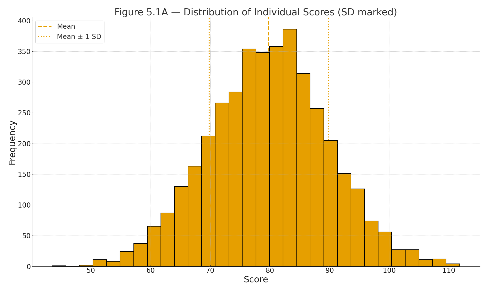
Visuals

Figure 5.1A — Distribution of individual scores with mean and ±1 SD marked.

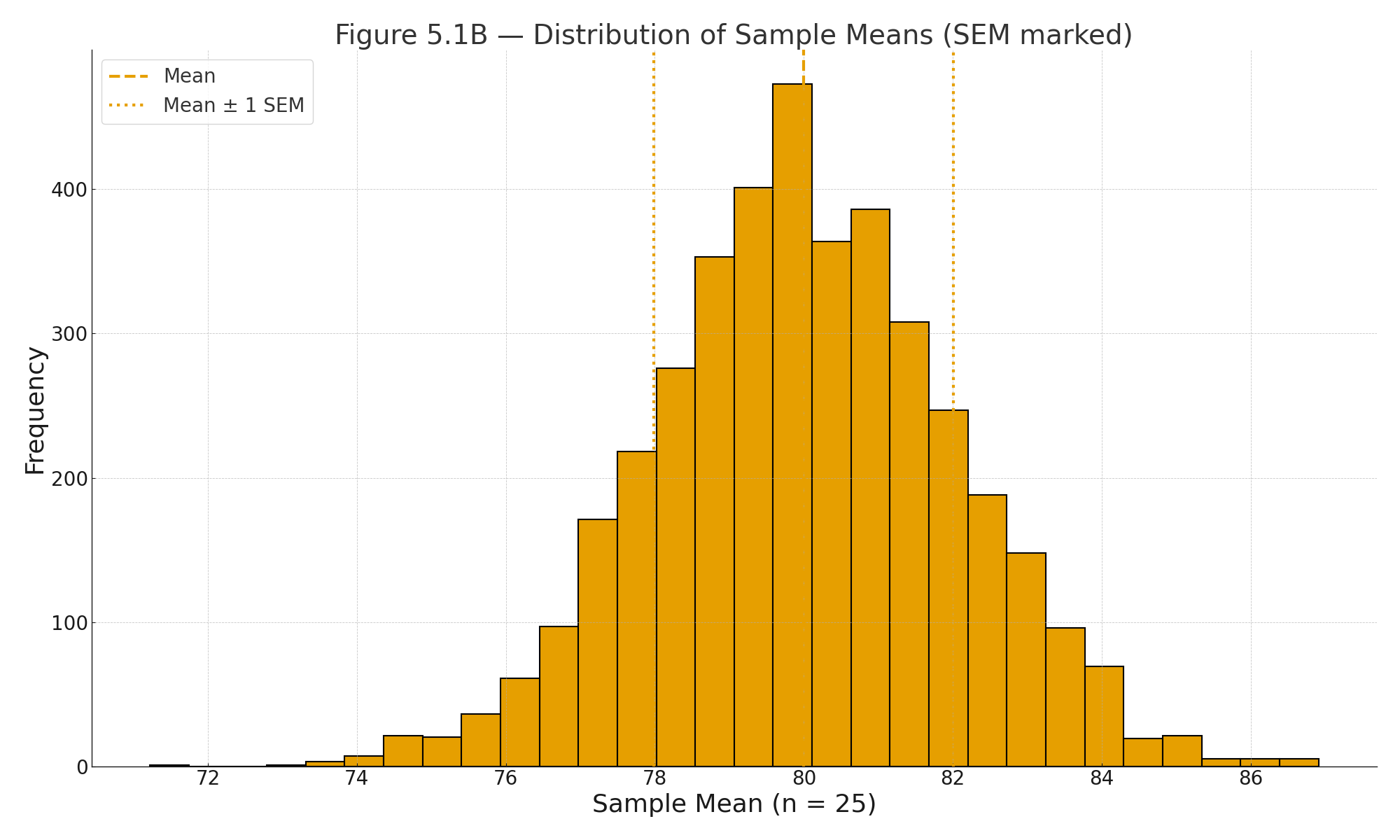
Figure 5.1B — Distribution of sample means (n = 25) with mean and ±1 SEM marked; note the narrower spread.

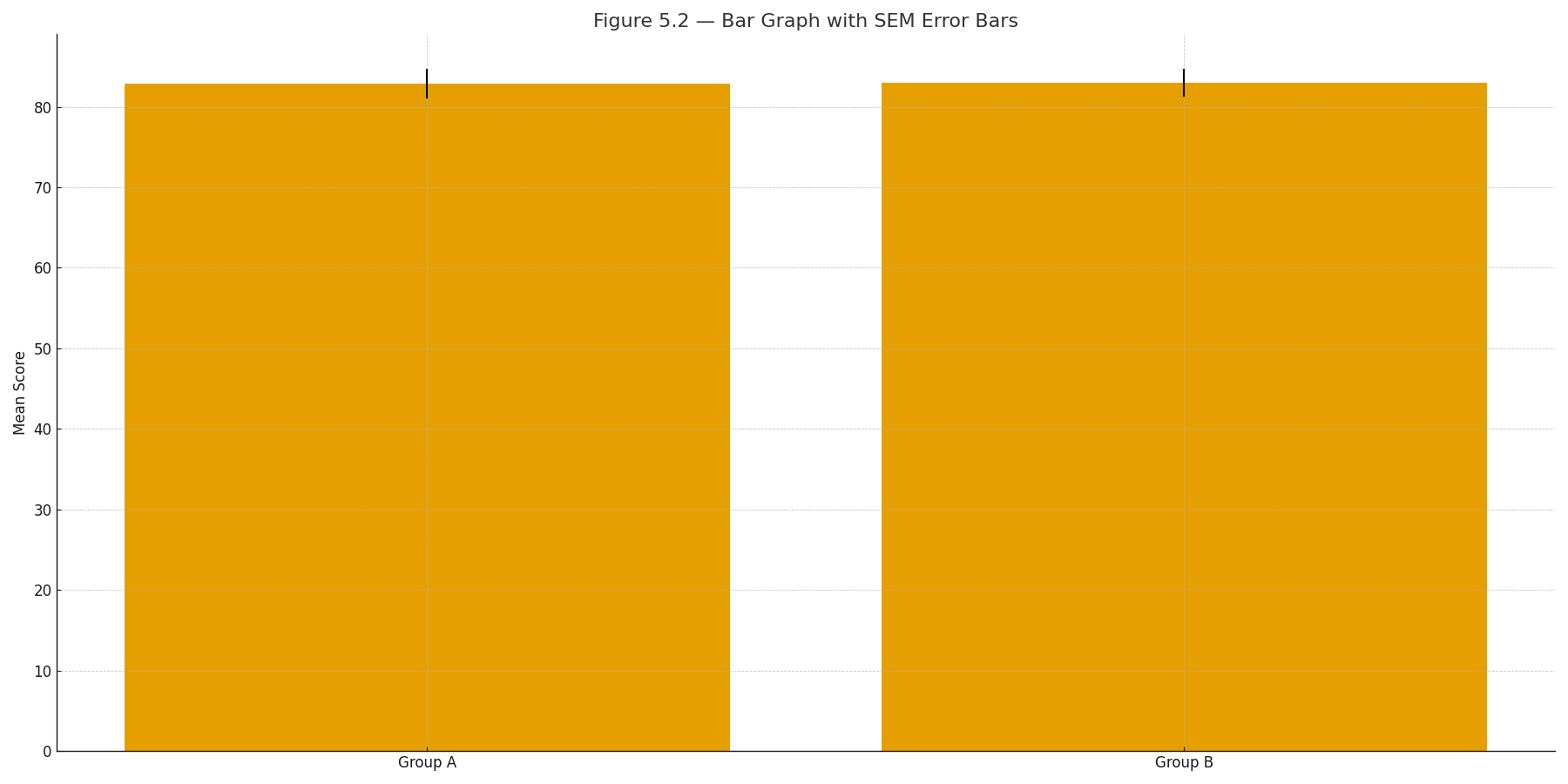
Figure 5.2 — Bar graph of two group means with error bars = SEM.

• It shows how reliable our sample mean is as an estimate of the population mean.
• A smaller SEM means a more precise estimate.
• The SEM appears in formulas for confidence intervals and t-tests.

Practice self-test quiz

In the space below, please find practice problems and self-test quizzes. For full access, please signup free.

The normal curve (bell curve) is one of the most important shapes in statistics. It appears when many small, independent factors combine: height, test scores, measurement errors.

For a simple, intuitive presentation go to Part 2

Properties of the Normal Curve

1. Symmetrical around the mean
2. Unimodal (one peak)
3. Mean = Median = Mode
4. The total area under the curve = 1 (or 100%)

Formula for the Normal Distribution

Unless you are in Mathematical Statistics, you will never be asked to reproduce it, or otherwise work with it.

Symbolic formula:
$$f(x) = \frac{1}{\sigma \sqrt{2\pi}} e^{-\frac{(x - \mu)^2}{2\sigma^2}}$$

Formula in words:
$$\text{Probability density} = \frac{1}{\text{standard deviation} \times \sqrt{2\pi}} \times e^{-\frac{(\text{score} - \text{mean})^2}{2 \times (\text{standard deviation})^2}}$$

Where:

• $$\mu$$ = mean
• $$\sigma$$ = standard deviation
• $$x$$ = a value on the curve

Standardization (z-scores)

Symbolic formula:
$$z = \frac{x - \mu}{\sigma}$$

Formula in words:
$$z = \frac{\text{score} - \text{mean}}{\text{standard deviation}}$$

A z-score tells us how many standard deviations a score is above or below the mean.

Key Percentages

Under the normal curve:

• About 68% of scores are within 1 standard deviation of the mean
• About 95% are within 2 standard deviations
• About 99.7% are within 3 standard deviations

This is called the 68–95–99.7 rule.

Example

Suppose test scores are normally distributed with

• $$\mu = 100$$
• $$\sigma = 15$$

What is the z-score for a student who scored 115?

$$z = \frac{115 - 100}{15} = \frac{15}{15} = 1$$

This means the student is 1 standard deviation above the mean.

Visuals

Figure 4.1 — The Normal Curve. A bell-shaped curve centered at the mean (μ).

Figure 4.2 — The 68–95–99.7 Rule. A normal curve with shaded regions for ±1σ, ±2σ, ±3σ.

Figure 4.3 — z-Score Example. Normal curve with shaded area to the left of z = 1.0, labeled 0.8413.

Why This Matters

The normal curve is the foundation of inferential statistics.

• It allows us to compute probabilities.
• It underlies the t-test, ANOVA, and confidence intervals.
• By using z-scores, we can compare scores across different tests and distributions.

Practice self-test quiz

In the space below, please find practice problems and self-test quizzes. For full access, please signup free.

Statistics is the science of learning from data. It provides the tools to decide whether what we observe is real or accidental, and whether a difference is large enough to matter.

When a scientist runs an experiment, or when a pollster surveys a group of voters, the results always vary. Statistics gives us a way to interpret that variation and to draw conclusions.

The Two Branches of Statistics

• Descriptive Statistics describe and summarize what we see.
  Example: “The average score on the math test was 78.”
• Inferential Statistics use a sample to make conclusions about a larger group.
  Example: “Based on this sample, we estimate the average score for all students in the district.”

Definition:

• Descriptive statistics = picture of the data.
• Inferential statistics = prediction about the population.

Parametric vs. Non-parametric Statistics

There are two main families of tests:

• Parametric tests (such as the t-test or ANOVA) assume certain conditions in the data, like normal distribution and interval/ratio measurement.
• Non-parametric tests (such as Chi-square or Mann–Whitney) require fewer assumptions and are used when data are ranks (ordinal) or categories (nominal).

Simple rule of thumb:

• If data are interval or ratio (e.g., test scores, heights), use parametric tests.
• If data are ordinal or nominal (e.g., ranks, categories), use non-parametric tests.

First Formula in Statistics: The Mean

The mean is our first step toward summarizing data.

Symbolic formula:
$$\bar{X} = \frac{\sum X}{n}$$

Formula in words:
$$\text{Mean} = \frac{\text{sum of scores}}{\text{number of scores}}$$

Where:

• $$\bar{X}$$ = mean (X bar)
• $$\sum X$$ = sum of all scores
• $$n$$ = number of scores

Example: Data: 6, 8, 10

$$\bar{X} = \frac{6 + 8 + 10}{3} = \frac{24}{3} = 8$$

So the mean is 8.

Visual

Figure 1.1 — The First Decision in Statistics. A flowchart: Descriptive vs. Inferential → Parametric vs. Non-parametric, with examples inside each box.

Why This Matters

Before you can choose the right statistical test, you must know:

1. What kind of data you have (descriptive vs. inferential).
2. How those data are measured (nominal, ordinal, interval, ratio).
3. Which family of tests applies (parametric vs. non-parametric).

This chapter sets the stage. The rest of the book builds from here, using only a small set of simple formulas to unlock the logic of statistics.

Practice self-test quiz

In the space below, please find practice problems and self-test quizzes. For full access, please signup free.