Welcome to Part 5 — Statistical Tests (Cookbook Style) of this free online high school statistics textbook. This practical quick-reference section provides concise, cookbook-style guides to major parametric and non-parametric statistical tests, including detailed formulas, assumptions, degrees of freedom, step-by-step procedures, and real-world examples. High school students and teachers can quickly review when to use each test—perfect for AP Statistics exam preparation, homework help, or reinforcing concepts from earlier parts.
Ideal for quick lookups on ANOVA variants, non-parametric alternatives, and multi-group comparisons, Part 5 delivers clear explanations of one-way ANOVA, factorial ANOVA, repeated-measures ANOVA, mixed ANOVA, Mann-Whitney U, Wilcoxon, Kruskal-Wallis, and Friedman tests in an accessible format with worked examples.
Statistical Tests Covered in Part 5
- One-Way ANOVA – Comparing means across three or more independent groups, with formula, degrees of freedom, and example.
- Factorial ANOVA (Two-Way) – Analyzing main effects and interactions in 2×2 or larger designs, including df partition and example.
- Repeated-Measures ANOVA – Handling multiple measurements on the same subjects, with formula and example.
- Mixed (Split-Plot) ANOVA – Combining between-subjects and within-subjects factors, with formula and example.
- Mann-Whitney U Test – Non-parametric alternative for two independent samples, with formula and example.
- Wilcoxon Signed-Rank Test – Non-parametric option for paired or one-sample data, with procedure and example.
- Kruskal-Wallis Test – Non-parametric one-way ANOVA for three or more groups, with formula and example.
- Friedman Test – Non-parametric repeated-measures ANOVA, with formula and example.
A practice self-test quiz is available to test your understanding (optional signup for full interactive access). Use this free high school statistics resource as your go-to cookbook for statistical tests formulas, ANOVA examples, non-parametric tests guides, and quick reference during hypothesis testing!
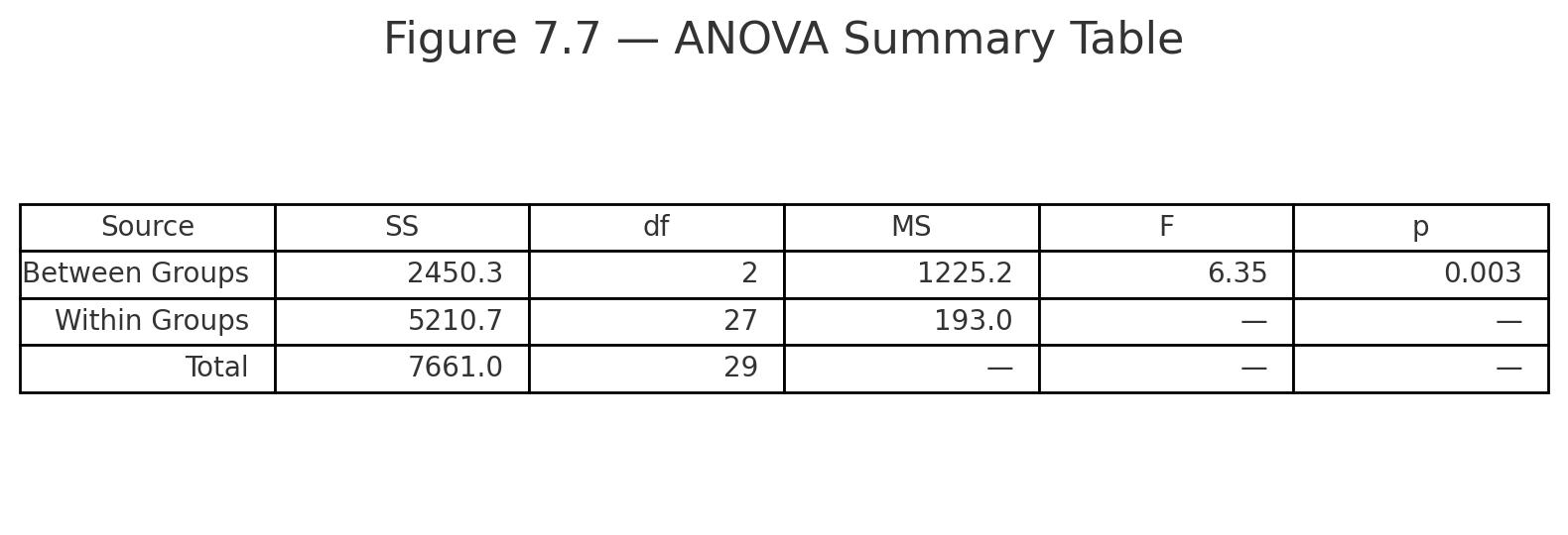
One-way ANOVA
When to Use:
- Compare means across 3 or more independent groups.
- Interval/ratio data, groups independent, variances roughly equal.
Formula:
$$F = \frac{MS_{\text{between}}}{MS_{\text{within}}}$$
In words:
$$F = \frac{\text{mean square between groups}}{\text{mean square within groups}}$$
Example:
Three groups with means = 70, 75, 85.
- $$SS_{\text{between}} = 300, , df_{\text{between}} = 2, , MS_{\text{between}} = 150$$
- $$SS_{\text{within}} = 200, , df_{\text{within}} = 12, , MS_{\text{within}} = 16.7$$
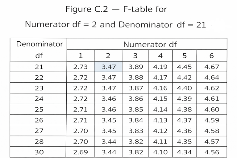
$$F = \frac{150}{16.7} = 9.0, \quad df = (2, 12)$$
Factorial ANOVA (Two-way)
When to Use:
- Two or more factors studied at once.
- Tests main effects and interactions.
Formula (df partition):
- $$df_A = a - 1, \quad df_B = b - 1$$
- $$df_{A \times B} = (a-1)(b-1)$$
- $$df_{\text{within}} = N - ab$$
Example:
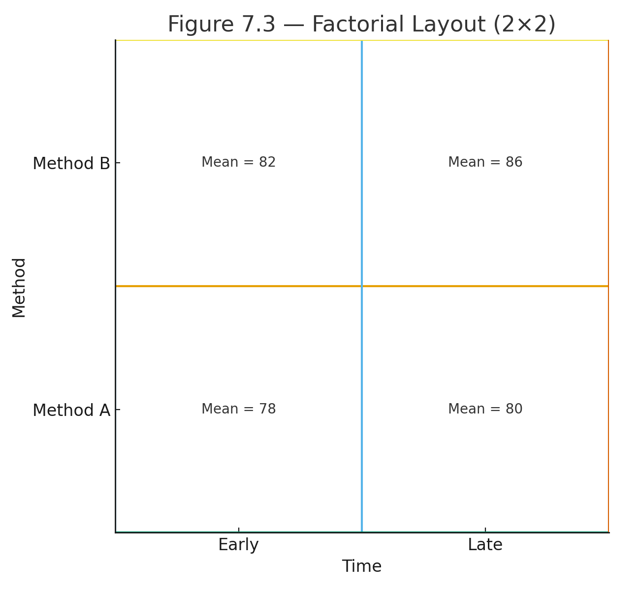
2 × 2 design (Method: Lecture, Online × Time: Morning, Afternoon).
- Lecture: Morning = 70, Afternoon = 90
- Online: Morning = 80, Afternoon = 80
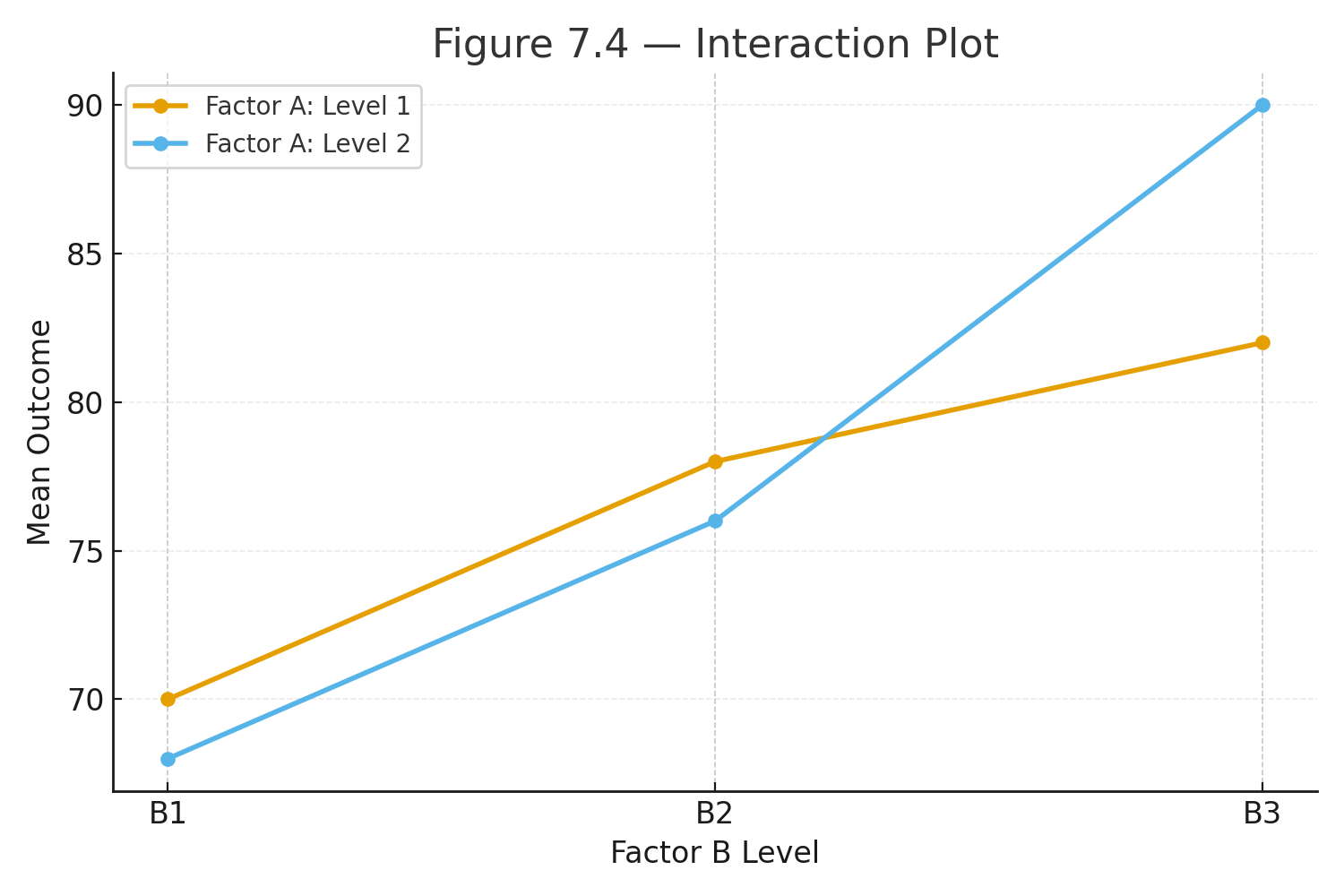
Interaction: Lecture improves over time, Online flat → non-parallel lines.
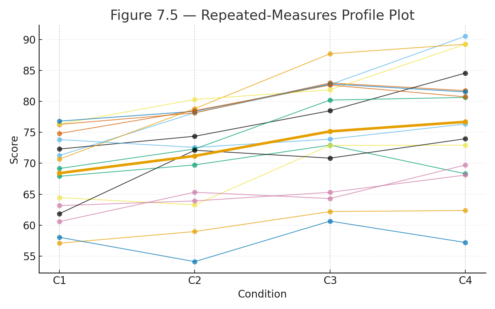
Repeated-Measures ANOVA
When to Use:
- Same participants tested under multiple conditions.
- Controls for subject variability.
Formula:
$$F = \frac{MS_{\text{conditions}}}{MS_{\text{error}}}$$
Degrees of Freedom:
- $$df_{\text{rows}} = n - 1$$
- $$df_{\text{columns}} = k - 1$$
- $$df_{\text{error}} = (n-1)(k-1)$$
Example:
Five students tested across 3 conditions. Mean scores rise steadily from 70 → 75 → 80.
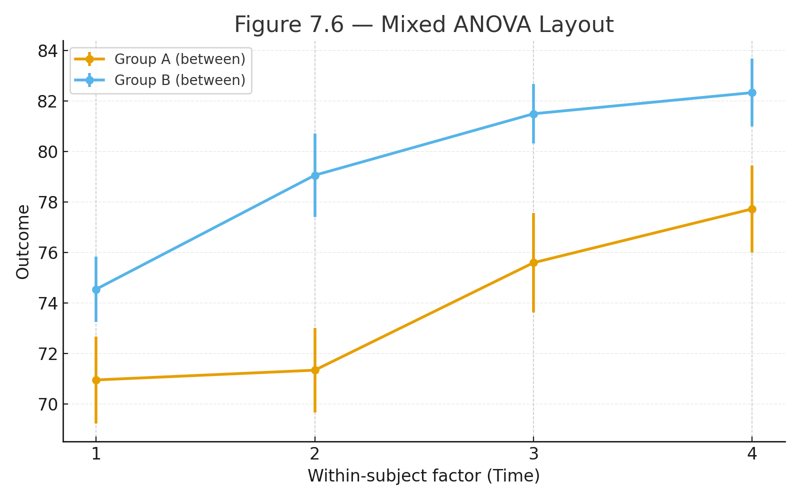
Mixed (Split-Plot) ANOVA
When to Use:
- Combines a between-subjects factor with a within-subjects factor.
- Common in psychology and education.
Formula (general):
$$F = \frac{MS_{\text{effect}}}{MS_{\text{error}}}$$
Degrees of Freedom:
- $$df_{\text{between}} = a - 1$$
- $$df_{\text{subjects}} = N - a$$
- $$df_{\text{within}} = b - 1$$
- $$df_{A \times B} = (a-1)(b-1)$$
Example:
Two groups (Drug, Placebo) × three weeks (repeated).
Drug scores rise each week, Placebo flat → interaction.
Mann–Whitney U Test
When to Use:
- Compare two independent groups when data are ordinal or not normally distributed.
- Non-parametric alternative to independent t-test.
Formula:
$$U = n_1 n_2 + \frac{n_1 (n_1 + 1)}{2} - R_1$$
Where $$R_1$$ = sum of ranks for group 1.
Example:
Two classrooms ranked by teacher ratings. Test whether distributions differ.
Wilcoxon Signed-Rank Test
When to Use:
- Compare the same group measured twice (before vs. after).
- Ordinal or non-normal data.
- Non-parametric alternative to paired t-test.
Procedure:
- Compute differences (After – Before).
- Rank absolute differences.
- Assign signs.
- Test statistic = smaller of the two signed sums.
Example:
Five students’ skill ranks before vs. after training. Test whether median rank improved.
Kruskal–Wallis Test
When to Use:
- Compare 3+ independent groups when data are ordinal or non-normal.
- Non-parametric alternative to one-way ANOVA.
Formula:
$$H = \frac{12}{N(N+1)} \sum \frac{R_j^2}{n_j} - 3(N+1)$$
Where:
- $$R_j$$ = sum of ranks for group j
- $$n_j$$ = number of observations in group j
- $$N$$ = total number of observations
Example:
Three therapy groups (n = 10 each) ranked by improvement scores.
Friedman Test
When to Use:
- Compare 3+ related groups (repeated measures, ordinal data).
- Non-parametric alternative to repeated-measures ANOVA.
Formula:
$$Q = \frac{12}{nk(k+1)} \sum R_j^2 - 3n(k+1)$$
Where:
- $$R_j$$ = sum of ranks for each condition
- $$n$$ = number of subjects
- $$k$$ = number of conditions
Example:
Ten students ranked across 3 types of training tasks.
Practice self-test quiz
In the space below, please find practice problems and self-test quizzes. For full access, please signup free.