hypothesis-testing

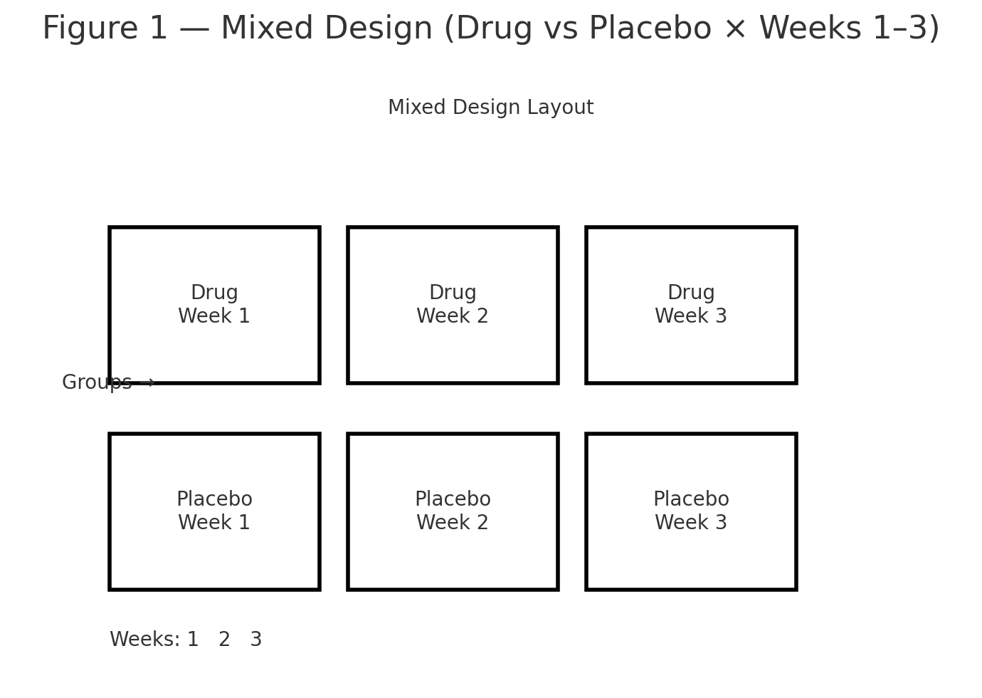
Goal. Test a between-subjects factor (Group: Drug vs. Placebo) and a within-subjects factor (Time: Weeks 1–3), plus their interaction, on exam scores.

Design & Experiment

• Between-subjects factor: Group = {Drug, Placebo}
• Within-subjects factor: Time = {Week 1, Week 2, Week 3}
• Balanced: 8 participants per group (\(s_g=8\)), 3 repeated measures per participant (\(k=3\)).

Participants are randomly assigned to Drug or Placebo. The same exam is given at Week 1, Week 2, and Week 3.

Figure 1: Mixed design layout (Drug vs Placebo × Weeks 1–3).

Data

Group: Drug (8 participants × 3 weeks)

Group: Placebo (8 participants × 3 weeks)

Totals. Grand sum = 1790 + 1704 = 3494, total observations \(N = 16\times3 = 48\), grand mean \( \bar X = 3494/48 = 72.7917\).

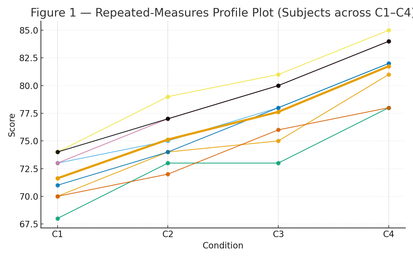
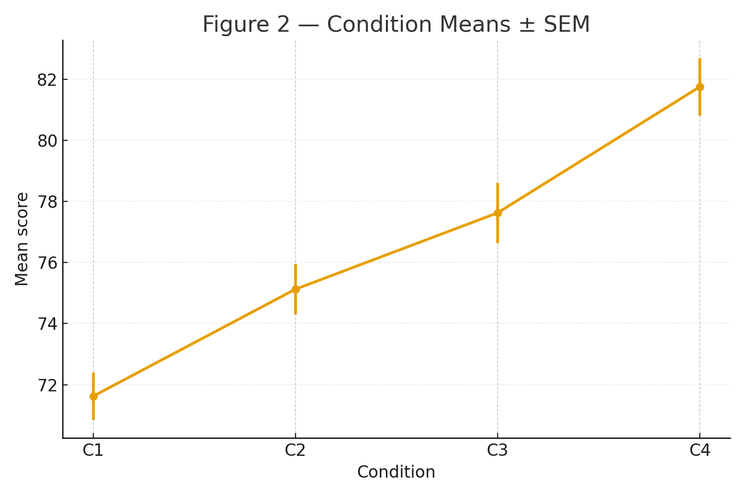
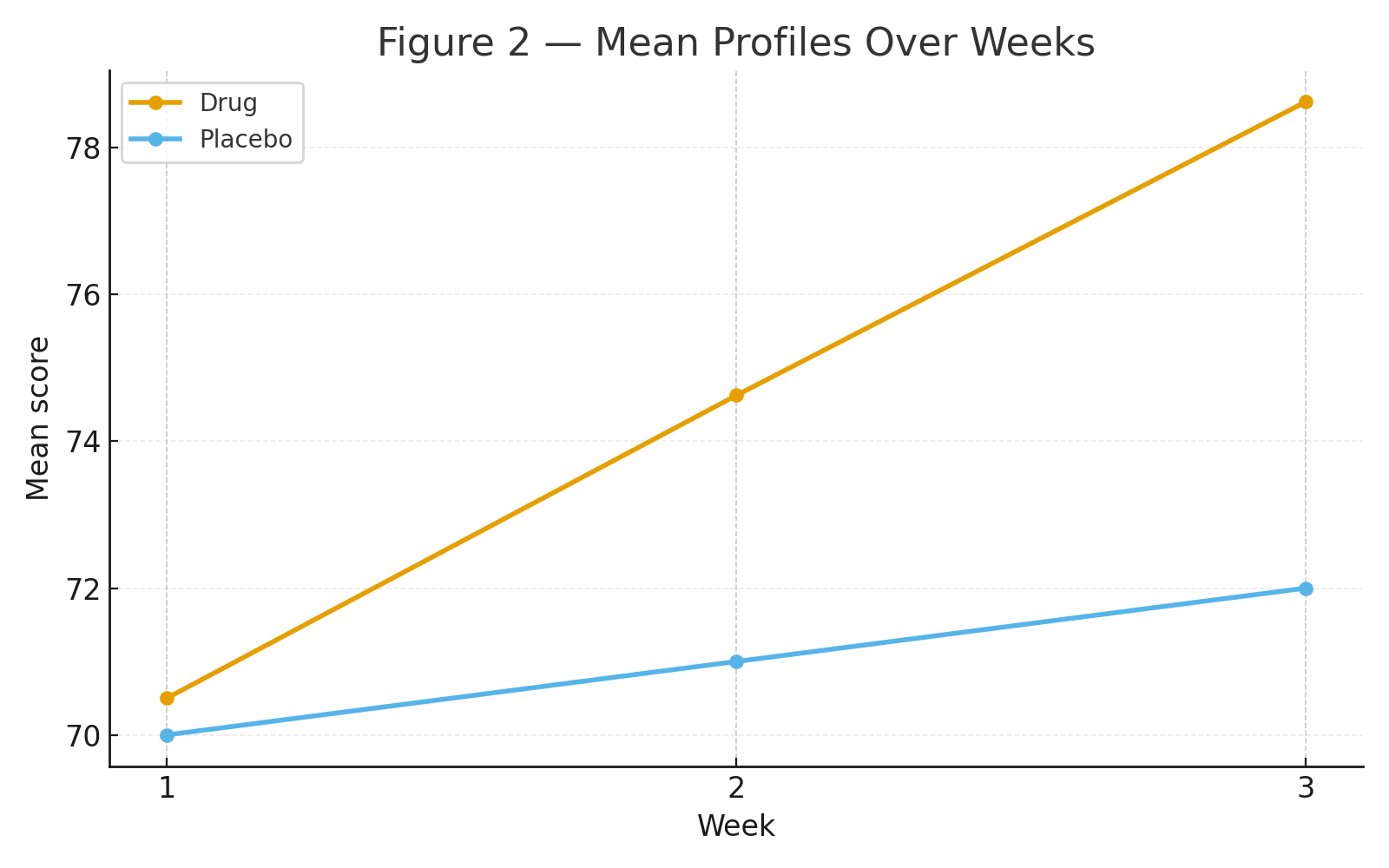
Figure 2: Mean profiles over weeks (Drug rises sharply; Placebo ~ flat).

Step 1 — Marginal Means

By Time (across both groups; 16 participants each week): \[ \bar X_{\text{W1}}=\tfrac{1124}{16}=70.2500,\qquad \bar X_{\text{W2}}=\tfrac{1165}{16}=72.8125,\qquad \bar X_{\text{W3}}=\tfrac{1205}{16}=75.3125, \] where column sums are \(1124, 1165, 1205\).

By Group (across all weeks): \[ \bar X_{\text{Drug}}=74.5833,\qquad \bar X_{\text{Placebo}}=71.0000. \]

Step 2 — Sums of Squares (SS)

Decompose total variability into Between-Subjects and Within-Subjects parts.

2A. Total

\[ SS_{\text{total}}=\sum (X_{igt}-\bar X)^2=\mathbf{527.9167}. \]

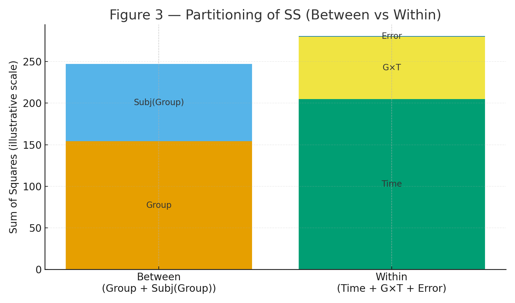
2B. Between-Subjects

Let each subject’s mean be \(\bar X_{i\cdot}\). Then \[ SS_{\text{BS-total}}=k\sum_{i=1}^{16}(\bar X_{i\cdot}-\bar X)^2=\mathbf{247.2500}. \] Split into Group and Subjects-within-Group: \[ SS_{\text{Group}}=k\sum_{g} n_g(\bar X_{g\cdot\cdot}-\bar X)^2=\mathbf{154.0833}, \] \[ SS_{\text{Subj}(g)}=k\sum_{i\in g}(\bar X_{i\cdot}-\bar X_{g\cdot\cdot})^2=\mathbf{93.1667}. \]

2C. Within-Subjects

\(SS_{\text{WS-total}}=SS_{\text{total}}-SS_{\text{BS-total}}=\mathbf{280.6667}.\)

Decompose into Time, Group×Time, and residual Error: \[ SS_{\text{Time}}=s\sum_{t}(\bar X_{\cdot\cdot t}-\bar X)^2=\mathbf{205.0417}, \] \[ SS_{\text{Group}\times\text{Time}} =\sum_{g,t} n_g\Big(\bar X_{g\cdot t}-\bar X_{g\cdot\cdot}-\bar X_{\cdot\cdot t}+\bar X\Big)^2 =\mathbf{75.0417}, \] \[ SS_{\text{Error(WS)}}=SS_{\text{WS-total}}-SS_{\text{Time}}-SS_{\text{G}\times\text{T}} =\mathbf{0.5833}. \]

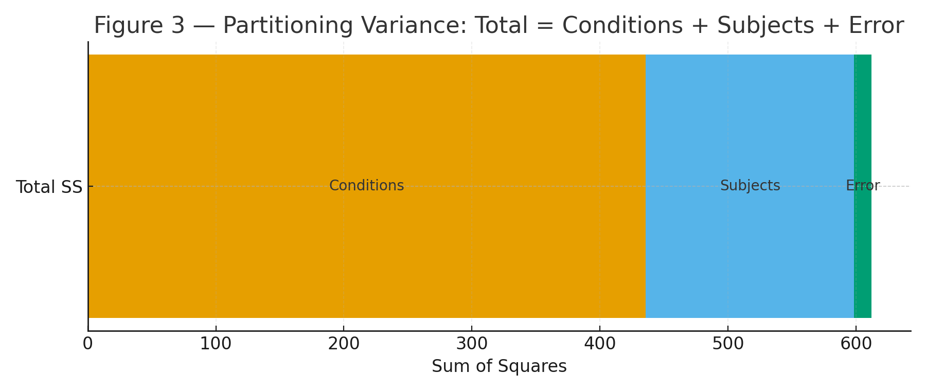
Figure 3: Partitioning diagram (Between: Group + Subj(Group); Within: Time + G×T + Error).

Step 3 — Degrees of Freedom (df) & Mean Squares (MS)

\[ \begin{aligned} &df_{\text{Group}}=g-1=1,\qquad df_{\text{Subj}(g)}=N_s-g=16-2=14,\\ &df_{\text{Time}}=k-1=2,\qquad df_{\text{G}\times\text{T}}=(g-1)(k-1)=2,\\ &df_{\text{Error(WS)}}=(N_s-g)(k-1)=(16-2)\times2=28,\\ &df_{\text{Total}}=Nk-1=48-1=47. \end{aligned} \]

\[ \begin{aligned} &MS_{\text{Group}}=\frac{SS_{\text{Group}}}{df_{\text{Group}}}= \frac{154.0833}{1}= \mathbf{154.0833},\qquad MS_{\text{Subj}(g)}=\frac{93.1667}{14}= \mathbf{6.6548},\\ &MS_{\text{Time}}=\frac{205.0417}{2}= \mathbf{102.5208},\qquad MS_{\text{G}\times\text{T}}=\frac{75.0417}{2}= \mathbf{37.5208},\\ &MS_{\text{Error(WS)}}=\frac{0.5833}{28}= \mathbf{0.02083}. \end{aligned} \]

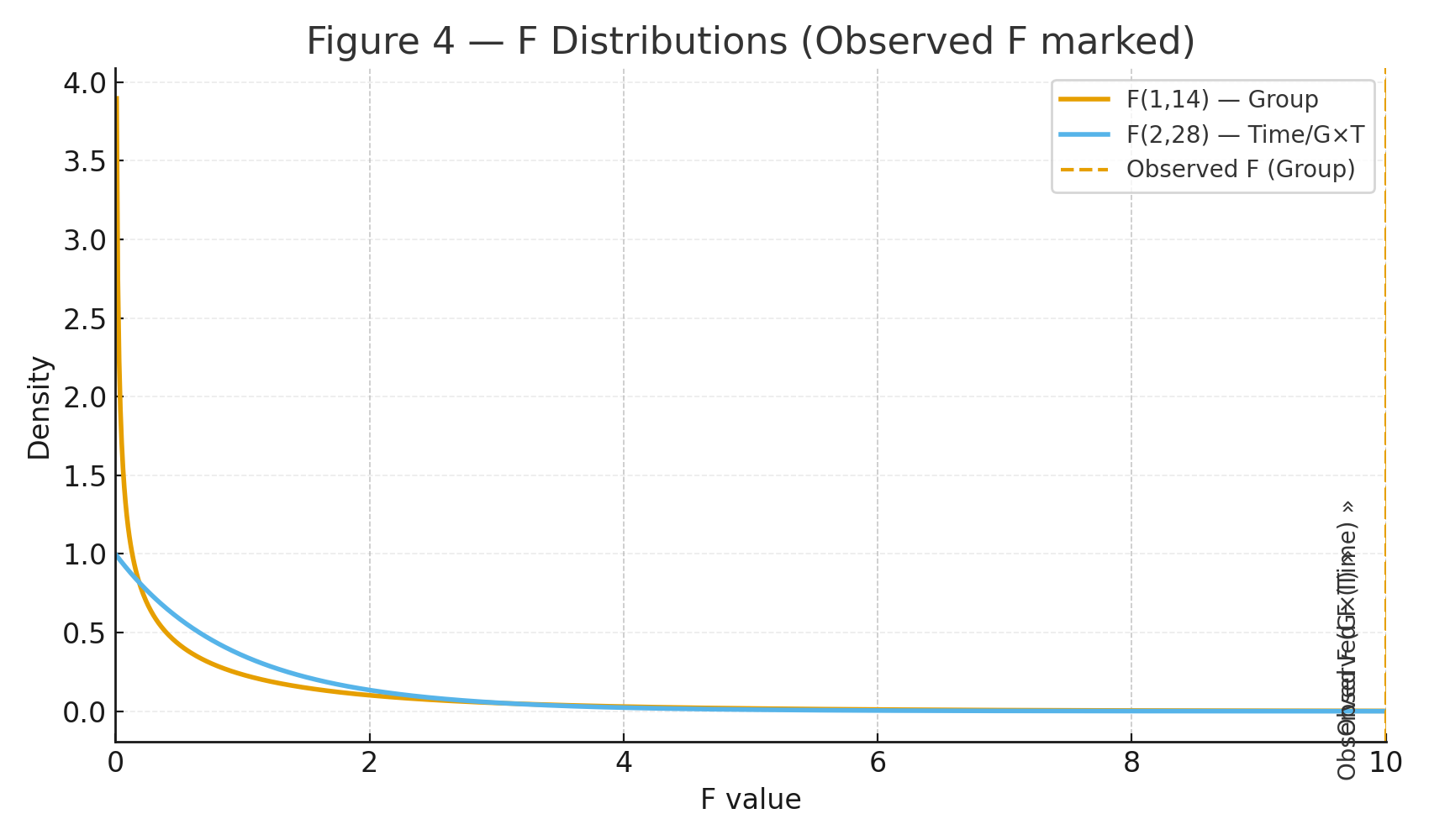
Step 4 — F Tests & p-values

Between-subjects test: \[ F_{\text{Group}}=\frac{MS_{\text{Group}}}{MS_{\text{Subj}(g)}}=\frac{154.0833}{6.6548}= \mathbf{23.1538}, \quad df=(1,14),\quad p\approx \mathbf{0.00028}. \]

Within-subjects tests: \[ F_{\text{Time}}=\frac{MS_{\text{Time}}}{MS_{\text{Error(WS)}}} =\frac{102.5208}{0.02083}= \mathbf{4921.0},\quad df=(2,28),\quad p\ll 10^{-20}. \] \[ F_{\text{G}\times\text{T}}=\frac{MS_{\text{G}\times\text{T}}}{MS_{\text{Error(WS)}}} =\frac{37.5208}{0.02083}= \mathbf{1801.0},\quad df=(2,28),\quad p\ll 10^{-20}. \]

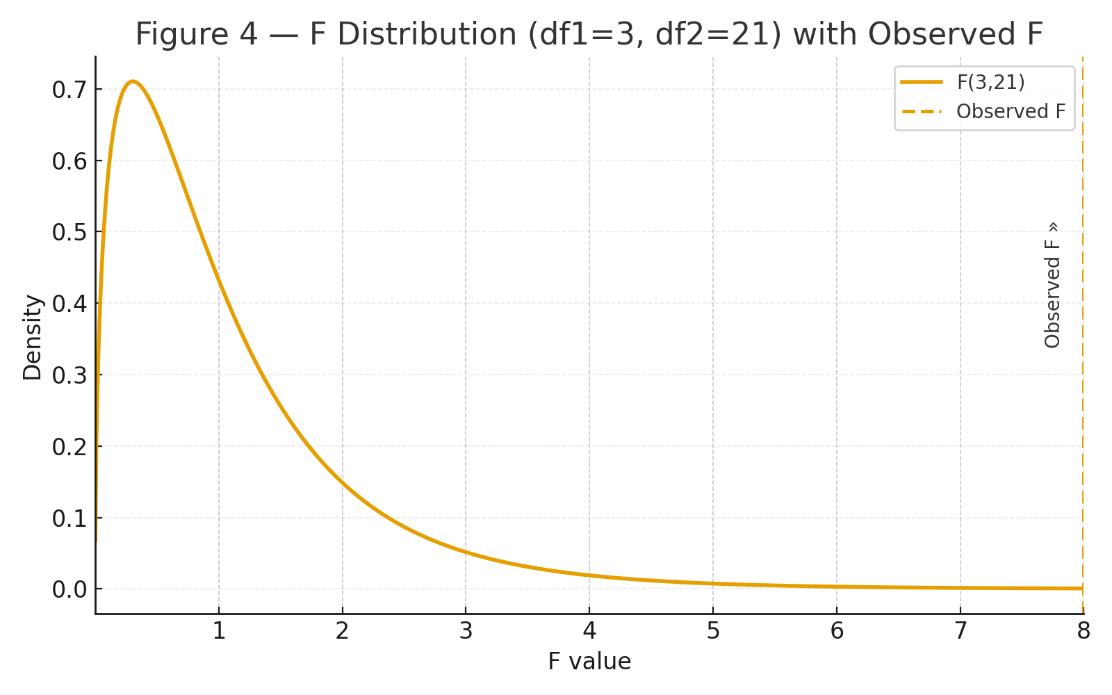
Figure 4: F distributions with observed statistics marked.

Mixed ANOVA Summary Table

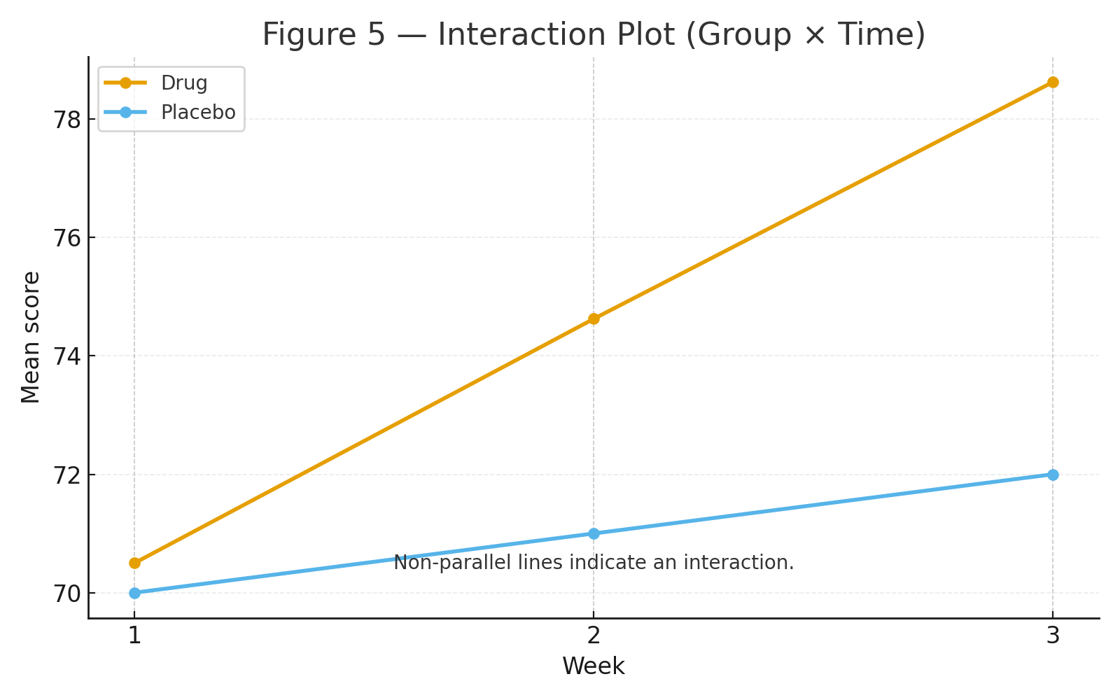
Interpretation

Group: Drug > Placebo overall (significant between-subjects effect).
Time: Scores increase across weeks (strong within-subjects effect).
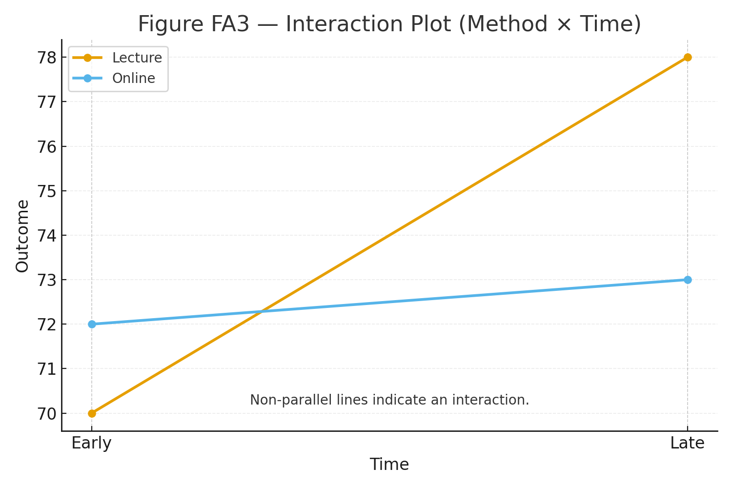
Group × Time: The Drug group improves sharply week-to-week while the Placebo group changes little (significant interaction).

Figure 5: Interaction plot showing non-parallel lines (Drug rising; Placebo flat).

Assumptions (checklist)

• Independence between subjects; correct grouping.
• Approximate normality within each Group×Time cell.
• Homogeneity of variance across groups (between-subjects).
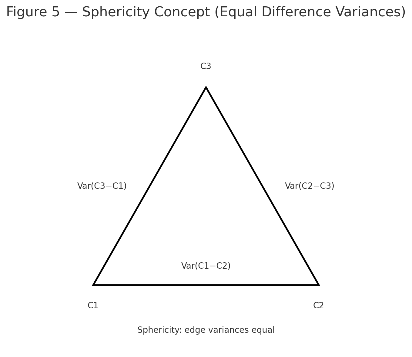
• Sphericity for the within-subject factor Time (apply Greenhouse–Geisser/Huynh–Feldt corrections if violated).

Note: The residual within-subject error is intentionally small in this teaching dataset, so the Time and G×T F values are very large. Real data typically have larger residual variability.

Practice self-test quiz

In the space below, please find practice problems and self-test quizzes. For full access, please signup free.

Goal. Test whether performance changes across four conditions measured on the same participants.

Design & Experiment

• Within-subjects factor: Condition with 4 levels (C1, C2, C3, C4).
• s = 8 participants measured in k = 4 conditions ⇒ total observations \(N = s \times k = 32\).
• Example context: the same students take four weekly quizzes after different study activities.

Figure 1: Profile plot (each subject as a line across the four conditions).

Data

Scores (rows = participants S1–S8; columns = conditions C1–C4):

Figure 2: Means ± SEM for C1–C4 (bar/line).

Step 1 — Condition Means (and sample variances)

\[ \begin{aligned} \bar X_{\mathrm{C1}} &= 573/8 = 71.625, \quad & s^2_{\mathrm{C1}} &= 4.8393 \\ \bar X_{\mathrm{C2}} &= 601/8 = 75.125, \quad & s^2_{\mathrm{C2}} &= 5.5536 \\ \bar X_{\mathrm{C3}} &= 621/8 = 77.625, \quad & s^2_{\mathrm{C3}} &= 7.6964 \\ \bar X_{\mathrm{C4}} &= 654/8 = 81.750, \quad & s^2_{\mathrm{C4}} &= 7.0714 \end{aligned} \]

Step 2 — Sums of Squares

Notation: \(s=8\) subjects, \(k=4\) conditions, grand mean \( \bar X = 76.53125\).

2A. Total

\[ SS_{\text{total}}=\sum_{i=1}^{s}\sum_{j=1}^{k}\bigl(X_{ij}-\bar X\bigr)^2 =\mathbf{611.96875}. \]

2B. Conditions (Treatment)

\[ SS_{\text{cond}}= s \sum_{j=1}^{k}\bigl(\bar X_{\cdot j}-\bar X\bigr)^2 = 8 \left[(71.625-76.53125)^2 + (75.125-76.53125)^2 + (77.625-76.53125)^2 + (81.75-76.53125)^2\right] =\mathbf{435.84375}. \]

2C. Subjects

\[ SS_{\text{subj}}= k \sum_{i=1}^{s}\bigl(\bar X_{i\cdot}-\bar X\bigr)^2 = 4 \sum_{i=1}^{8}\bigl(\bar X_{i\cdot}-76.53125\bigr)^2 =\mathbf{162.71875}. \]

2D. Error (Residual)

\[ SS_{\text{error}}= SS_{\text{total}} - SS_{\text{cond}} - SS_{\text{subj}} = 611.96875 - 435.84375 - 162.71875 =\mathbf{13.40625}. \]

Figure 3: Partitioning variance diagram (Total → Conditions + Subjects + Error).

Step 3 — Degrees of Freedom & Mean Squares

\[ \begin{aligned} df_{\text{cond}} &= k-1 = 3, \\ df_{\text{subj}} &= s-1 = 7, \\ df_{\text{error}} &= (s-1)(k-1) = 7\times3 = 21, \\ df_{\text{total}} &= sk-1 = 31. \end{aligned} \]

\[ MS_{\text{cond}} = \frac{SS_{\text{cond}}}{df_{\text{cond}}} =\frac{435.84375}{3}=\mathbf{145.28125},\qquad MS_{\text{error}} = \frac{SS_{\text{error}}}{df_{\text{error}}} =\frac{13.40625}{21}=\mathbf{0.6383928571}. \]

Step 4 — Test Statistic & p-value

\[ F = \frac{MS_{\text{cond}}}{MS_{\text{error}}} = \frac{145.28125}{0.6383928571} =\mathbf{227.5734}. \] With \(df_1=3\) and \(df_2=21\), this is extremely large. The right-tail p-value is effectively \(p \lt 10^{-12}\) (i.e., \(p \ll .001\)).

Figure 4: F distribution with observed F marked and right-tail region shaded.

Repeated-Measures ANOVA Summary Table

Interpretation

Mean performance increases steadily from C1 → C4, and the repeated-measures ANOVA shows a highly significant effect of Condition, \(F(3,21)=227.57,\, p\ll .001\). Follow-ups (e.g., paired t-tests with Bonferroni/Holm) can localize which pairs of conditions differ.

Assumptions (checklist)

• Sphericity (equal variances of the differences between condition pairs). If violated, apply Greenhouse–Geisser or Huynh–Feldt correction to \(df\).
• Approximately normal scores within each condition.
• No carryover/fatigue effects that confound order (counterbalancing helps).

Figure 5: Sphericity concept sketch (pairwise difference variances).

Practice self-test quiz

In the space below, please find practice problems and self-test quizzes. For full access, please signup free.

Goal. Test the effects of Method (Lecture vs. Online) and Time (Early vs. Late) on exam scores, and whether there is an interaction between Method and Time.

Design & Experiment

• Factor A (Method): Lecture vs. Online
• Factor B (Time): Early vs. Late
• Balanced design: \(n=5\) per cell ⇒ total \(N=20\).

Students are randomly assigned to one of four cells (Method × Time). After a short module, all students take the same 100-point exam.

Figure 1: 2 × 2 layout (Method × Time).

Data

Scores by cell (five students per cell):

Within each cell the sample variance is 4 (SD = 2), so the within-cell sum of squares is \((n-1)s^2 = 4\times4 = 16\) per cell.

Figure 2: Means with SEM by Time, separate lines for Method.

Figure 3: Interaction plot (Lecture rises sharply; Online nearly flat).

Step 1 — Marginal Means and Grand Mean

Cell means: \[ \bar X_{\text{Lecture,Early}}=70,\; \bar X_{\text{Lecture,Late}}=78,\; \bar X_{\text{Online,Early}}=72,\; \bar X_{\text{Online,Late}}=73. \] Marginal means: \[ \bar X_{\text{Lecture}}=\frac{70+78}{2}=74,\quad \bar X_{\text{Online}}=\frac{72+73}{2}=72.5; \qquad \bar X_{\text{Early}}=\frac{70+72}{2}=71,\quad \bar X_{\text{Late}}=\frac{78+73}{2}=75.5. \] Grand mean: \[ \bar X=\frac{70+78+72+73}{4}=73.25. \]

Step 2 — Sums of Squares (Between)

Balanced design formulas (with \(n\) per cell, \(a=b=2\)):

• \(SS_A = nb \sum_a(\bar X_{a\cdot}-\bar X)^2\), here \(nb=10\).
• \(SS_B = na \sum_b(\bar X_{\cdot b}-\bar X)^2\), here \(na=10\).
• \(SS_{AB} = n \sum_{a,b}\big(\bar X_{ab}-\bar X_{a\cdot}-\bar X_{\cdot b}+\bar X\big)^2\), here \(n=5\).

Compute each term:

Factor A (Method): \[ \begin{aligned} SS_A &= 10\Big[(74-73.25)^2 + (72.5-73.25)^2\Big]\\ &= 10\big[0.75^2 + (-0.75)^2\big] = 10(0.5625+0.5625)=\mathbf{11.25}. \end{aligned} \]

Factor B (Time): \[ \begin{aligned} SS_B &= 10\Big[(71-73.25)^2 + (75.5-73.25)^2\Big]\\ &= 10\big[(-2.25)^2 + (2.25)^2\big] = 10(5.0625+5.0625)=\mathbf{101.25}. \end{aligned} \]

Interaction \(A\times B\): For each cell compute \(d_{ab}=\bar X_{ab}-\bar X_{a\cdot}-\bar X_{\cdot b}+\bar X\). Here each \(d_{ab}=\pm1.75\) so \(d_{ab}^2=3.0625\) and there are four cells: \[ SS_{AB}=5\times(4\times3.0625)=\mathbf{61.25}. \]

Step 3 — Within-Group (Error) and Total SS

Within each cell, \((n-1)s^2=16\). With 4 cells: \[ SS_{\text{within}}=\mathbf{64.00}. \]

Total: \[ SS_{\text{total}}=SS_A+SS_B+SS_{AB}+SS_{\text{within}} =11.25+101.25+61.25+64.00=\mathbf{238.75}. \]

Step 4 — Degrees of Freedom & Mean Squares

\[ \begin{aligned} &df_A=a-1=1,\quad df_B=b-1=1,\quad df_{AB}=(a-1)(b-1)=1,\\ &df_{\text{within}}=N-ab=20-4=\mathbf{16},\quad df_{\text{total}}=N-1=19. \end{aligned} \] \[ MS_A=\frac{11.25}{1}=11.25,\quad MS_B=\frac{101.25}{1}=101.25,\quad MS_{AB}=\frac{61.25}{1}=61.25,\quad MS_{\text{within}}=\frac{64.00}{16}=\mathbf{4.00}. \]

Step 5 — F Tests & p-values

\[ F_A=\frac{MS_A}{MS_{\text{within}}}=\frac{11.25}{4}= \mathbf{2.8125},\qquad F_B=\frac{MS_B}{MS_{\text{within}}}=\frac{101.25}{4}= \mathbf{25.3125},\qquad F_{AB}=\frac{MS_{AB}}{MS_{\text{within}}}=\frac{61.25}{4}= \mathbf{15.3125}. \] With \(df_1=1\), \(df_2=16\): \[ p_A \approx 0.11\;(\text{n.s.}),\quad p_B < 0.001,\quad p_{AB} \approx 0.001. \]

ANOVA Summary Table

Interpretation

Main effect of Time (B) is significant: Late > Early on average. Main effect of Method (A) is not significant at conventional levels. The interaction (A × B) is significant: Lecture improves markedly from Early→Late, while Online changes little—non-parallel lines in the interaction plot.

Figure 4: Interaction plot highlighting non-parallel lines.

Assumptions (checklist)

• Independence of observations within and across cells.
• Approximately normal scores within each cell.
• Homogeneity of variances across cells (here, each cell variance ≈ 4).

Practice self-test quiz

In the space below, please find practice problems and self-test quizzes. For full access, please signup free.

The z-table gives areas (probabilities) under the standard normal curve (mean $$\mu=0$$, SD $$\sigma=1$$).
Use it after you standardize a score:

Standardization (z-score):
$$z=\frac{x-\mu}{\sigma}$$
In words: $$z=\frac{\text{score} - \text{mean}}{\text{standard deviation}}$$

What the z-table shows

Most tables list the area to the left of a z value (cumulative probability).

• Left area at $$z=0$$ is 0.5000 (half the curve).
• Far left (negative big z) approaches 0; far right (positive big z) approaches 1.

Quick recipes

1) Probability below a score (left tail)
Example: $$z=1.00$$ → table gives 0.8413.
Interpretation: $$P(Z \le 1.00)=0.8413$$ (84.13% below).

2) Probability above a score (right tail)
Use complement: $$P(Z \ge z)=1-\text{left area}$$.
Example: $$z=1.00 \Rightarrow P(Z \ge 1.00)=1-0.8413=0.1587.$$

3) Probability between two scores
Subtract left areas.
Example: between $$z= -0.50$$ (left area 0.3085) and $$z=1.20$$ (0.8849):
$$P(-0.50 \le Z \le 1.20)=0.8849-0.3085=0.5764.$$

4) From a raw score to probability
Test scores: $$\mu=100, \ \sigma=15$$. What % are below 115?
Standardize: $$z=\frac{115-100}{15}=1.00 \Rightarrow 0.8413 \ (\text{84.13%}).$$

5) From probability to raw score (percentile)
What score is the 90th percentile?
Find z with left area ≈ 0.9000 → $$z \approx 1.2816$$.
Convert back: $$x=\mu+z\sigma=100+(1.2816)(15)=119.22.$$

Tips

• For negative z, use the table’s symmetry: left area at $$-z$$ equals 1 − left area at $$+z$$.
• Rounding: two decimals is common (e.g., 1.23).
• Modern tools (calculator/Sheets/Python) can give exact p-values directly.

Visuals

Figure D.1 — Normal curve with area left of z = 1.00 shaded (0.8413).
Figure D.2 — Two-z shaded band for “between” probability.

📱 QR: Online z-calculator (type z or x, get areas instantly)

Practice self-test quiz

In the space below, please find practice problems and self-test quizzes. For full access, please signup free.

Tables give the critical values we compare our test statistic against.
They depend on:

• The significance level (α, often 0.05)
• The degrees of freedom (df)

t-table

• Rows = degrees of freedom (df)
• Columns = significance level (α)

Example:

• Independent-samples t-test with n₁ = 12, n₂ = 12
• df = 12 + 12 – 2 = 22
• At α = 0.05 (two-tailed) → critical t ≈ 2.07
• If $$|t| \geq 2.07$$ → significant

F-table

• Needs two df values:
  • df between (numerator)
  • df within (denominator)

Example:

• One-way ANOVA, 3 groups, N = 24
• df between = k – 1 = 2
• df within = N – k = 21
• At α = 0.05 → critical F ≈ 3.47
• If computed F ≥ 3.47 → significant

Student Tips

• Always compute df correctly.
• Use tables if no software is available.
• Most calculators or apps today give exact p-values — faster than tables.

📱 QR: Interactive critical value calculator (t and F tables online)

Visuals

Figure C.1 — Snippet of a t-table row (df = 22, α = 0.05 highlighted).
Figure C.2 — F-table grid with numerator df = 2, denominator df = 21 marked.

Practice self-test quiz

In the space below, please find practice problems and self-test quizzes. For full access, please signup free.

Classical statistics uses formulas and tables.
Modern computing gives us another way: resampling and simulation.

Instead of relying only on theory, we let the computer generate thousands of samples and see what happens.

Bootstrapping

Bootstrapping means resampling with replacement from the original data.

Steps:

1. Take a sample of size $$n$$ from the data (with replacement).
2. Compute the statistic (mean, median, correlation).
3. Repeat thousands of times.
4. Use the distribution of resampled statistics to estimate confidence intervals.

Example:
Data = [5, 6, 7, 9].
Resample 1000 times, compute mean each time.
The distribution of means gives an estimate of the true mean’s variability.

Randomization (Permutation) Tests

Used to test hypotheses by shuffling labels.

Steps:

1. Combine all data.
2. Randomly assign to groups.
3. Compute the difference in means.
4. Repeat thousands of times.
5. Compare the observed difference to this distribution.

This shows whether the observed effect could be due to chance.

Monte Carlo Simulation

Monte Carlo methods use random numbers to model complex processes.

Example: Estimating $$\pi$$.

• Randomly throw points into a square.
• Count how many fall inside the circle quarter.
• $$\pi \approx 4 \times \tfrac{\text{inside circle}}{\text{total points}}$$.

Why Resampling Works

Resampling uses the data itself as a model of the population.
It avoids assumptions (like normality) and adapts to modern computing power.

Visuals

Figure 15.1 — Bootstrapping illustration: resampling from a small dataset with replacement.

Figure 15.2 — Randomization test: labels shuffled between groups.

Figure 15.3 — Monte Carlo: random points filling a square and a quarter circle.

Why This Matters

Resampling and simulation show students that statistics is not only about formulas.
Computers allow us to see probability in action.
This approach prepares students for data science, where simulation is as important as theory.

Practice self-test quiz

In the space below, please find practice problems and self-test quizzes. For full access, please signup free.

Every statistical test requires degrees of freedom (df).
Degrees of freedom tell us how many independent pieces of information are available once totals or means are fixed.
They determine which row of the t-table or F-table we use.

General rule:

$$df = \text{number of observations} - \text{number of constraints}$$

t-tests

• One-sample t-test:
  $$df = n - 1$$
• Independent-samples t-test:
  $$df = n_1 + n_2 - 2$$
• Paired-samples t-test:
  $$df = n - 1$$

One-way ANOVA

• Between groups:
  $$df_{\text{between}} = k - 1$$
• Within groups:
  $$df_{\text{within}} = N - k$$
• Total:
  $$df_{\text{total}} = N - 1$$

Where $$k$$ = number of groups, $$N$$ = total number of scores.

Factorial ANOVA (2 × 2 Example)

• Factor A: $$df_A = a - 1$$
• Factor B: $$df_B = b - 1$$
• Interaction: $$df_{A \times B} = (a-1)(b-1)$$
• Error: $$df_{\text{within}} = N - ab$$

Repeated-Measures ANOVA

• Rows (subjects): $$df_{\text{rows}} = n - 1$$
• Columns (conditions): $$df_{\text{columns}} = k - 1$$
• Error: $$df_{\text{error}} = (n - 1)(k - 1)$$

Where $$n$$ = number of subjects, $$k$$ = number of conditions.

Mixed (Split-Plot) ANOVA

• Between factor: $$df_{\text{between}} = a - 1$$
• Subjects within groups: $$df_{\text{subjects}} = N - a$$
• Within factor: $$df_{\text{within}} = b - 1$$
• Interaction: $$df_{A \times B} = (a-1)(b-1)$$

Chi-square

• Goodness-of-fit: $$df = k - 1$$
• Independence: $$df = (r - 1)(c - 1)$$

Where $$k$$ = number of categories, $$r$$ = rows, $$c$$ = columns.

Visuals

Variables: \( n \)=sample size, \( n_1,n_2 \)=group sizes, \( N \)=total scores, \( k \)=# of groups/conditions, \( a,b \)=levels of factors A,B, \( r,c \)=rows, columns.

Why This Matters

Degrees of freedom link sample size to critical values.
They tell us how much room for variability exists in the data.
With this quick cookbook, you can locate the right df for any test.

Practice self-test quiz

In the space below, please find practice problems and self-test quizzes. For full access, please signup free.

The chi-square test ($$\chi^2$$) is used with categorical (nominal) data.
It compares observed frequencies with expected frequencies.

Chi-square Goodness-of-Fit

When to Use:

• One categorical variable
• Test if observed frequencies match expected frequencies

Formula:
$$\chi^2 = \sum \frac{(O - E)^2}{E}$$

In words:
$$\chi^2 = \text{sum of squared differences between observed and expected, divided by expected}$$

Example:
Survey of favorite subjects (Math, Science, English).
Expected = equal (⅓ each), Observed = [25, 30, 45].
Compute each (O–E)²/E, sum = χ².

Chi-square Test of Independence

When to Use:

• Two categorical variables
• Test whether they are associated (independent or not)

Formula:
$$\chi^2 = \sum \frac{(O - E)^2}{E}$$

Where expected frequencies:
$$E = \frac{(\text{row total})(\text{column total})}{\text{grand total}}$$

Example:
Gender (Male/Female) × Sport (Soccer/Basketball/Tennis).
If observed counts differ from expected, χ² tests independence.

Chi-square Correlation Measures

Chi-square can also give a measure of association strength between categorical variables.

• Phi coefficient (φ): for 2 × 2 tables

$$\phi = \sqrt{\frac{\chi^2}{N}}$$

• Cramer’s V: for larger tables

$$V = \sqrt{\frac{\chi^2}{N(k-1)}}$$

Where $$k = \min(\text{rows}, \text{columns})$$.

• Contingency coefficient (C):

$$C = \sqrt{\frac{\chi^2}{\chi^2 + N}}$$

Example (Phi, Cramer’s V, Contingency C)

Suppose χ² = 10.0, N = 100.

• For 2 × 2: $$\phi = \sqrt{10/100} = \sqrt{0.1} = 0.32$$
• For 3 × 2 table: $$V = \sqrt{10/(100(2-1))} = \sqrt{0.1} = 0.32$$
• Contingency coefficient: $$C = \sqrt{10/(10+100)} = \sqrt{0.09} = 0.30$$

Definition

• Goodness-of-fit: one categorical variable vs. expected distribution
• Independence: relationship between two categorical variables
• Correlation measures: strength of association in categorical tables (φ, V, C)

Visuals

Figure 12.1 — Goodness-of-fit example: observed vs. expected bar chart.

Figure 12.2 — Independence test: 2 × 2 contingency table with expected values.

Figure 12.3 — Phi, Cramer’s V, and C illustrated with 2 × 2 and 3 × 2 tables.

Why This Matters

Chi-square lets us analyze data that are counts rather than scores.
It extends statistical testing beyond numbers into categories — essential for psychology, sociology, education, and medicine.

Practice self-test quiz

In the space below, please find practice problems and self-test quizzes. For full access, please signup free.

Welcome to Part 5 — Statistical Tests (Cookbook Style) of this free online high school statistics textbook. This practical quick-reference section provides concise, cookbook-style guides to major parametric and non-parametric statistical tests, including detailed formulas, assumptions, degrees of freedom, step-by-step procedures, and real-world examples. High school students and teachers can quickly review when to use each test—perfect for AP Statistics exam preparation, homework help, or reinforcing concepts from earlier parts.

Ideal for quick lookups on ANOVA variants, non-parametric alternatives, and multi-group comparisons, Part 5 delivers clear explanations of one-way ANOVA, factorial ANOVA, repeated-measures ANOVA, mixed ANOVA, Mann-Whitney U, Wilcoxon, Kruskal-Wallis, and Friedman tests in an accessible format with worked examples.

Statistical Tests Covered in Part 5

1. One-Way ANOVA – Comparing means across three or more independent groups, with formula, degrees of freedom, and example.
2. Factorial ANOVA (Two-Way) – Analyzing main effects and interactions in 2×2 or larger designs, including df partition and example.
3. Repeated-Measures ANOVA – Handling multiple measurements on the same subjects, with formula and example.
4. Mixed (Split-Plot) ANOVA – Combining between-subjects and within-subjects factors, with formula and example.
5. Mann-Whitney U Test – Non-parametric alternative for two independent samples, with formula and example.
6. Wilcoxon Signed-Rank Test – Non-parametric option for paired or one-sample data, with procedure and example.
7. Kruskal-Wallis Test – Non-parametric one-way ANOVA for three or more groups, with formula and example.
8. Friedman Test – Non-parametric repeated-measures ANOVA, with formula and example.

A practice self-test quiz is available to test your understanding (optional signup for full interactive access). Use this free high school statistics resource as your go-to cookbook for statistical tests formulas, ANOVA examples, non-parametric tests guides, and quick reference during hypothesis testing!

One-way ANOVA

When to Use:

• Compare means across 3 or more independent groups.
• Interval/ratio data, groups independent, variances roughly equal.

Formula:
$$F = \frac{MS_{\text{between}}}{MS_{\text{within}}}$$

In words:
$$F = \frac{\text{mean square between groups}}{\text{mean square within groups}}$$

Example:
Three groups with means = 70, 75, 85.

• $$SS_{\text{between}} = 300, , df_{\text{between}} = 2, , MS_{\text{between}} = 150$$
• $$SS_{\text{within}} = 200, , df_{\text{within}} = 12, , MS_{\text{within}} = 16.7$$

$$F = \frac{150}{16.7} = 9.0, \quad df = (2, 12)$$

Factorial ANOVA (Two-way)

When to Use:

• Two or more factors studied at once.
• Tests main effects and interactions.

Formula (df partition):

• $$df_A = a - 1, \quad df_B = b - 1$$
• $$df_{A \times B} = (a-1)(b-1)$$
• $$df_{\text{within}} = N - ab$$

Example:
2 × 2 design (Method: Lecture, Online × Time: Morning, Afternoon).

• Lecture: Morning = 70, Afternoon = 90
• Online: Morning = 80, Afternoon = 80

Interaction: Lecture improves over time, Online flat → non-parallel lines.

Repeated-Measures ANOVA

When to Use:

• Same participants tested under multiple conditions.
• Controls for subject variability.

Formula:
$$F = \frac{MS_{\text{conditions}}}{MS_{\text{error}}}$$

Degrees of Freedom:

• $$df_{\text{rows}} = n - 1$$
• $$df_{\text{columns}} = k - 1$$
• $$df_{\text{error}} = (n-1)(k-1)$$

Example:
Five students tested across 3 conditions. Mean scores rise steadily from 70 → 75 → 80.

Mixed (Split-Plot) ANOVA

When to Use:

• Combines a between-subjects factor with a within-subjects factor.
• Common in psychology and education.

Formula (general):
$$F = \frac{MS_{\text{effect}}}{MS_{\text{error}}}$$

Degrees of Freedom:

• $$df_{\text{between}} = a - 1$$
• $$df_{\text{subjects}} = N - a$$
• $$df_{\text{within}} = b - 1$$
• $$df_{A \times B} = (a-1)(b-1)$$

Example:
Two groups (Drug, Placebo) × three weeks (repeated).
Drug scores rise each week, Placebo flat → interaction.

Mann–Whitney U Test

When to Use:

• Compare two independent groups when data are ordinal or not normally distributed.
• Non-parametric alternative to independent t-test.

Formula:
$$U = n_1 n_2 + \frac{n_1 (n_1 + 1)}{2} - R_1$$

Where $$R_1$$ = sum of ranks for group 1.

Example:
Two classrooms ranked by teacher ratings. Test whether distributions differ.

Wilcoxon Signed-Rank Test

When to Use:

• Compare the same group measured twice (before vs. after).
• Ordinal or non-normal data.
• Non-parametric alternative to paired t-test.

Procedure:

1. Compute differences (After – Before).
2. Rank absolute differences.
3. Assign signs.
4. Test statistic = smaller of the two signed sums.

Example:
Five students’ skill ranks before vs. after training. Test whether median rank improved.

Kruskal–Wallis Test

When to Use:

• Compare 3+ independent groups when data are ordinal or non-normal.
• Non-parametric alternative to one-way ANOVA.

Formula:
$$H = \frac{12}{N(N+1)} \sum \frac{R_j^2}{n_j} - 3(N+1)$$

Where:

• $$R_j$$ = sum of ranks for group j
• $$n_j$$ = number of observations in group j
• $$N$$ = total number of observations

Example:
Three therapy groups (n = 10 each) ranked by improvement scores.

Friedman Test

When to Use:

• Compare 3+ related groups (repeated measures, ordinal data).
• Non-parametric alternative to repeated-measures ANOVA.

Formula:
$$Q = \frac{12}{nk(k+1)} \sum R_j^2 - 3n(k+1)$$

Where:

• $$R_j$$ = sum of ranks for each condition
• $$n$$ = number of subjects
• $$k$$ = number of conditions

Example:
Ten students ranked across 3 types of training tasks.

Practice self-test quiz

In the space below, please find practice problems and self-test quizzes. For full access, please signup free.

Case 1 — Independent t-test (Two Groups)

Scenario: A teacher wants to compare math test scores between students taught with traditional lectures and those taught with interactive software.

Question: Are the two teaching methods different in average test score?

Design/Test: Independent-samples t-test.

Worked Example:

• Group A (Lecture): mean = 78, SD = 10, n = 20
• Group B (Software): mean = 85, SD = 12, n = 20

Formula:
$$t = \frac{\bar{X}_1 - \bar{X}_2}{\sqrt{\tfrac{s_1^2}{n_1} + \tfrac{s_2^2}{n_2}}}$$

In words:
$$t = \frac{\text{mean}_1 - \text{mean}_2}{\sqrt{\tfrac{\text{variance}_1}{n_1} + \tfrac{\text{variance}_2}{n_2}}}$$

Plugging in values:
$$t = \frac{78 - 85}{\sqrt{\tfrac{100}{20} + \tfrac{144}{20}}} = \frac{-7}{\sqrt{5 + 7.2}} = \frac{-7}{\sqrt{12.2}} = \frac{-7}{3.49} = -2.01$$

Degrees of freedom = 38.

Case 2 — Paired t-test (Before and After)

Scenario: Students take a memory test before and after a week of practice.

Question: Did memory scores improve after training?

Design/Test: Paired-samples t-test.

Worked Example:

Differences (After – Before): 2, 4, 3, 5, 6

• Mean difference:
  $$\bar{D} = \frac{2+4+3+5+6}{5} = 4$$
• Standard deviation of differences: $$s_D = 1.58$$

Formula:
$$t = \frac{\bar{D}}{s_D / \sqrt{n}}$$

Plugging in values:
$$t = \frac{4}{1.58/\sqrt{5}} = \frac{4}{0.71} = 5.63$$

Degrees of freedom = 4.

Case 3 — One-way ANOVA (Three Groups)

Scenario: A psychologist tests three methods of stress reduction: meditation, exercise, and music.

Question: Do the methods differ in average stress score?

Design/Test: One-way ANOVA.

Worked Example (summary):

• Group means: Meditation = 65, Exercise = 70, Music = 80
• $$SS_{\text{between}} = 300, , df_{\text{between}} = 2, , MS_{\text{between}} = 150$$
• $$SS_{\text{within}} = 200, , df_{\text{within}} = 12, , MS_{\text{within}} = 16.7$$

Formula:
$$F = \frac{MS_{\text{between}}}{MS_{\text{within}}}$$

Plugging in values:
$$F = \frac{150}{16.7} = 9.0$$

df = (2, 12).

Practice self-test quiz

In the space below, please find practice problems and self-test quizzes. For full access, please signup free.