```html

Appendix 6 — Data Sets for Practice

Working with real numbers is the best way to learn statistics. This appendix provides small “mini datasets” you can analyze by hand (or with a calculator), plus larger files for practice with spreadsheets.

Dataset Provenance (Read This First)

• Pedagogical = small, simplified numbers chosen to make learning and checking easier.
• Simulated = computer-generated numbers designed to resemble real data (not collected from real people).
• Empirical = collected from real observations (only used if explicitly stated).

Note: Unless a dataset is explicitly labeled Empirical, you should treat it as Pedagogical or Simulated practice data.

Mini Datasets (In-Page)

1) Quiz Scores

Provenance: Pedagogical
n: 10
Scale: Ratio (points)
Data: 6, 7, 8, 9, 10, 7, 8, 6, 9, 10

• Suggested Lessons:
  • Lesson 2 — The Averages: mean, median, mode
  • Lesson 3 — Variance & Standard Deviation: variance, SD, z-scores
  • Lesson 4 — The Standard Normal Curve: interpret z-scores (as a bridge)
• Check values (optional): Mean = 8.0; SD ≈ 1.41

2) Reaction Times (ms)

Provenance: Pedagogical (human-like values)
n: 8
Scale: Ratio (milliseconds)
Units: ms
Data: 220, 250, 270, 230, 260, 280, 240, 300

• Suggested Lessons:
  • Lesson 3 — Variance & Standard Deviation: spread, outliers, SD
  • Lesson 6 — The t-test: use as a template dataset (e.g., compare two conditions by splitting into two groups)
  • Lesson 7 — ANOVA: extend to 3+ groups by creating conditions
• Instructor tip: reaction time data often show mild skew in real life. If you want skew, see the larger practice files below.

3) Stress Reduction Scores (Three Groups)

Provenance: Pedagogical (grouped scores)
Scale: Interval/Ratio (score units; treat as interval for ANOVA practice)
Groups:

• Meditation (n = 3): 65, 70, 72
• Exercise (n = 3): 68, 71, 75
• Music (n = 3): 75, 78, 82
• Suggested Lessons:
  • Lesson 7 — ANOVA: one-way ANOVA (three independent groups)
  • Lesson 8 — Post Hoc Tests: follow-up comparisons after ANOVA (conceptual)
  • Lesson 13 — Degrees of Freedom Cookbook: df for one-way ANOVA
• Important note: The sample sizes are intentionally small for learning mechanics. In real studies, groups are usually larger.

Larger Practice Datasets (Download Files)

These datasets are designed for spreadsheet work, graphing, and full problem sets.

• Exam Scores (n = 100)
  Provenance: Simulated
  Suggested Lessons: Lesson 4 (normal curve), Lesson 5 (SEM), Lesson 6 (t-test foundations)
• Survey Data (preferences by gender/age)
  Provenance: Simulated (categorical practice)
  Suggested Lessons: Lesson 12 (chi-square), Lesson 1 (why statistics matters in decisions)
• Simulated Medical Trial (treatment vs. control, repeated measures)
  Provenance: Simulated (instructional “trial-style” dataset; not clinical research)
  Suggested Lessons: Lesson 6 (t-test concepts), Lesson 7 (variance partitioning concepts), and for advanced learners: repeated-measures ideas (optional)

Downloads: CSV and Excel files are provided via the QR code(s) on this page (and/or direct links, if enabled on your device).

Reproducibility note (simulated files): If you revise these datasets in future editions, consider generating them with a fixed random seed so instructors and students can reproduce results across versions.

Trusted External Sources (Optional)

If you want additional datasets beyond the practice files above, the following repositories are widely used for learning and benchmarking:

• NIST Statistical Reference Datasets (SRD)
  High-quality benchmark datasets for practice and verification (excellent for checking calculations and software).
• UCI Machine Learning Repository
  Larger, more complex datasets. Recommended only for advanced students or enrichment projects.

Visual Reference

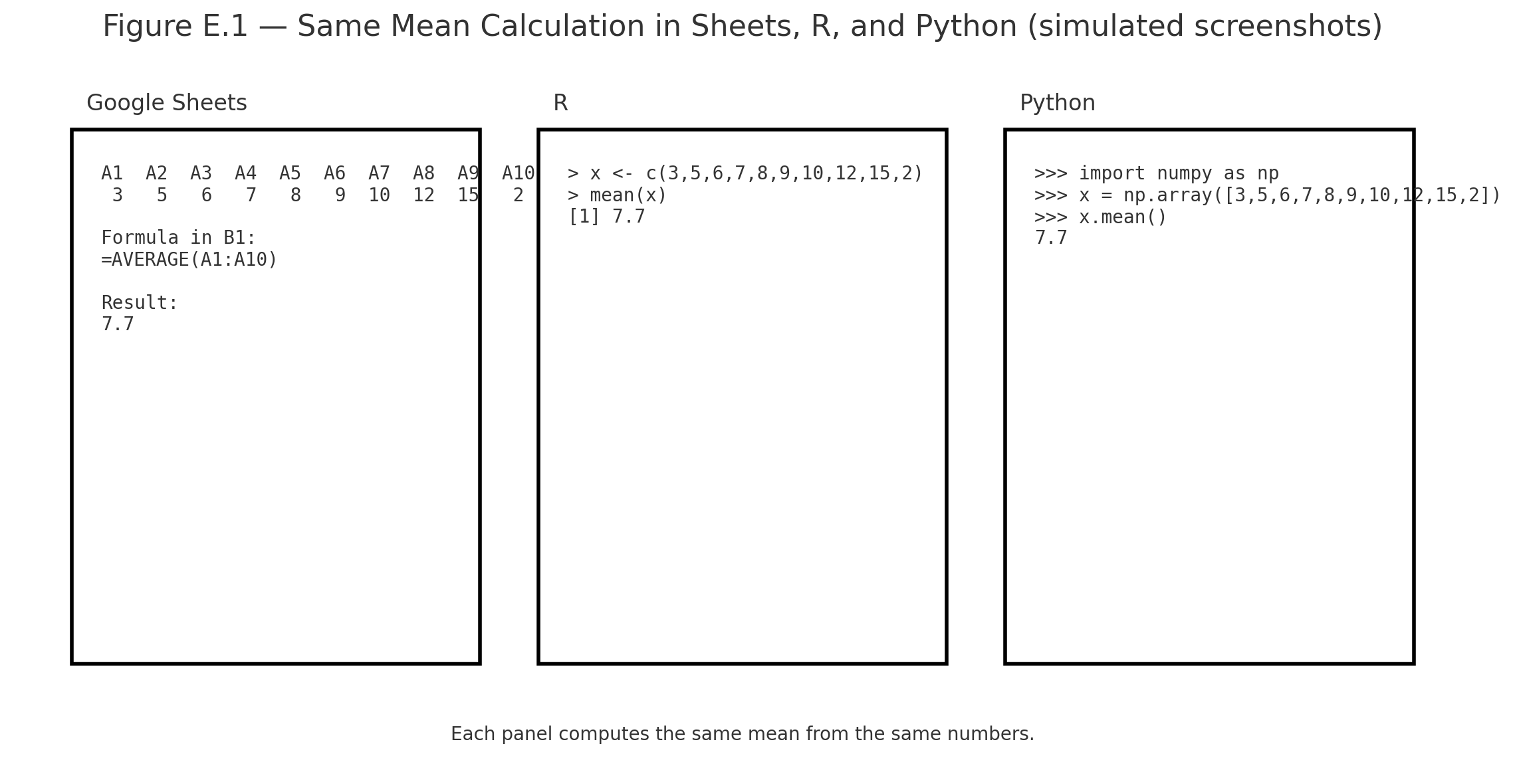
Figure F.1 — Example spreadsheet view of a dataset (columns such as ID, Score, Group). Use this as a template for organizing your own data before running calculations.

Self-Test Quiz Access

Practice problems and self-test quizzes may appear below. If full access is restricted, please sign up (free) to unlock the quiz section.

```

Statistics can be done with calculators, spreadsheets, or software. Here’s a quick guide.

Excel / Google Sheets

R (RStudio or RStudio Cloud)

Python (NumPy / SciPy / Pandas)

iPhone Calculator

• Rotate sideways → scientific mode
• Use √ for square root
• Parentheses matter: type numerator, then divide by denominator
• Fine for small problems, but not for full datasets

Summary

• For quick homework: iPhone calculator
• For assignments: Excel / Google Sheets
• For coding: Python (Colab) or R (RStudio Cloud)

📱 QR: Open sample data in Google Sheets (ready to practice mean, SD, t-test)

Visuals

Figure E.1 — Screenshots of the same mean calculation in Sheets, R, and Python side by side.

Practice self-test quiz

In the space below, please find practice problems and self-test quizzes. For full access, please signup free.

The z-table gives areas (probabilities) under the standard normal curve (mean $$\mu=0$$, SD $$\sigma=1$$).
Use it after you standardize a score:

Standardization (z-score):
$$z=\frac{x-\mu}{\sigma}$$
In words: $$z=\frac{\text{score} - \text{mean}}{\text{standard deviation}}$$

What the z-table shows

Most tables list the area to the left of a z value (cumulative probability).

• Left area at $$z=0$$ is 0.5000 (half the curve).
• Far left (negative big z) approaches 0; far right (positive big z) approaches 1.

Quick recipes

1) Probability below a score (left tail)
Example: $$z=1.00$$ → table gives 0.8413.
Interpretation: $$P(Z \le 1.00)=0.8413$$ (84.13% below).

2) Probability above a score (right tail)
Use complement: $$P(Z \ge z)=1-\text{left area}$$.
Example: $$z=1.00 \Rightarrow P(Z \ge 1.00)=1-0.8413=0.1587.$$

3) Probability between two scores
Subtract left areas.
Example: between $$z= -0.50$$ (left area 0.3085) and $$z=1.20$$ (0.8849):
$$P(-0.50 \le Z \le 1.20)=0.8849-0.3085=0.5764.$$

4) From a raw score to probability
Test scores: $$\mu=100, \ \sigma=15$$. What % are below 115?
Standardize: $$z=\frac{115-100}{15}=1.00 \Rightarrow 0.8413 \ (\text{84.13%}).$$

5) From probability to raw score (percentile)
What score is the 90th percentile?
Find z with left area ≈ 0.9000 → $$z \approx 1.2816$$.
Convert back: $$x=\mu+z\sigma=100+(1.2816)(15)=119.22.$$

Tips

• For negative z, use the table’s symmetry: left area at $$-z$$ equals 1 − left area at $$+z$$.
• Rounding: two decimals is common (e.g., 1.23).
• Modern tools (calculator/Sheets/Python) can give exact p-values directly.

Visuals

Figure D.1 — Normal curve with area left of z = 1.00 shaded (0.8413).
Figure D.2 — Two-z shaded band for “between” probability.

📱 QR: Online z-calculator (type z or x, get areas instantly)

Practice self-test quiz

In the space below, please find practice problems and self-test quizzes. For full access, please signup free.

Tables give the critical values we compare our test statistic against.
They depend on:

• The significance level (α, often 0.05)
• The degrees of freedom (df)

t-table

• Rows = degrees of freedom (df)
• Columns = significance level (α)

Example:

• Independent-samples t-test with n₁ = 12, n₂ = 12
• df = 12 + 12 – 2 = 22
• At α = 0.05 (two-tailed) → critical t ≈ 2.07
• If $$|t| \geq 2.07$$ → significant

F-table

• Needs two df values:
  • df between (numerator)
  • df within (denominator)

Example:

• One-way ANOVA, 3 groups, N = 24
• df between = k – 1 = 2
• df within = N – k = 21
• At α = 0.05 → critical F ≈ 3.47
• If computed F ≥ 3.47 → significant

Student Tips

• Always compute df correctly.
• Use tables if no software is available.
• Most calculators or apps today give exact p-values — faster than tables.

📱 QR: Interactive critical value calculator (t and F tables online)

Visuals

Figure C.1 — Snippet of a t-table row (df = 22, α = 0.05 highlighted).
Figure C.2 — F-table grid with numerator df = 2, denominator df = 21 marked.

Practice self-test quiz

In the space below, please find practice problems and self-test quizzes. For full access, please signup free.

Artificial Intelligence (AI) aims to build systems that can learn, adapt, and make decisions.
One powerful tool is the neural network, inspired by the brain.

From Statistics to AI

• Regression predicts Y from X
• Logistic regression predicts probability (0–1)
• Neural networks generalize this idea: many inputs, many layers, nonlinear patterns

The Structure of a Neural Network

1. Input layer — variables (X₁, X₂, …)
2. Hidden layers — units that transform the input
3. Output layer — prediction or classification

Each connection has a weight (like a slope in regression).

Formula for a Neuron

A single unit in the network:

$$z = \sum w_i X_i + b$$

$$y = f(z)$$

Where:

• $$w_i$$ = weights
• $$X_i$$ = inputs
• $$b$$ = bias (like an intercept)
• $$f(z)$$ = activation function (e.g., logistic, ReLU)

Learning in a Network

The network predicts outputs and compares them with the true answers.
The error is sent backward through the network to adjust weights.
This is called backpropagation.

Example

Predicting if a student will pass or fail based on:

• Study hours
• Attendance
• Practice problems completed

Inputs → combined with weights → logistic activation → output: probability of passing.

Visuals

Figure 18.1 — Simple Neural Network (Inputs → Hidden → Output)

Figure 18.2 — Activation Functions

Why This Matters

• Neural networks extend regression and logistic regression.
• They allow learning from large, complex datasets (images, speech, language).
• Modern AI (translation, recognition, chatbots) is powered by these models.

Practice self-test quiz

In the space below, please find practice problems and self-test quizzes. For full access, please signup free.

Simple regression predicts Y from one X.
But in real life, outcomes often depend on several variables — or may not be linear.

This chapter introduces multiple regression and logistic regression.

Multiple Regression

Formula:

$$\hat{Y} = a + b_1X_1 + b_2X_2 + \dots + b_kX_k$$

In words:
$$\text{Predicted Y} = \text{intercept} + (b_1 \times X_1) + (b_2 \times X_2) + \dots$$

Where:

• $$X_1, X_2, \dots X_k$$ = predictors
• $$b_1, b_2, \dots b_k$$ = slopes (weights for each predictor)

Example: Predicting college GPA from:

• High school GPA ($$X_1$$)
• Study hours ($$X_2$$)

Equation:
$$\hat{Y} = 1.0 + 0.5X_1 + 0.1X_2$$

Interpretation:

• For each 1-point increase in HS GPA, college GPA rises 0.5.
• For each extra study hour, GPA rises 0.1.

Coefficient of Determination

In multiple regression, $$R^2$$ tells us the proportion of variance explained by all predictors together.

Example: $$R^2 = 0.65$$ → predictors explain 65% of the outcome’s variability.

Logistic Regression

What if the outcome is yes/no (categorical)?
Example: Will a student pass or fail?

We use logistic regression.

Formula:

$$P(Y=1) = \frac{1}{1 + e^{-(a + bX)}}$$

In words:
$$\text{Probability of success} = \frac{1}{1 + e^{-(\text{intercept} + \text{slope} \times X)}}$$

Output: probability between 0 and 1.

Example: Predicting pass/fail from study hours.

• Equation: $$P = \frac{1}{1 + e^{-( -2 + 0.5X )}}$$
• If X = 6 hours: $$P = \frac{1}{1 + e^{-1}} = 0.73$$
• About 73% chance of passing.

Visuals

Figure 17.1 — Multiple regression plane: Y predicted from two predictors.

Figure 17.2 — Logistic regression curve: probability vs. study hours.

Why This Matters

• Multiple regression = prediction with many factors
• Logistic regression = prediction when the outcome is categorical
• $$R^2$$ = strength of prediction

These methods expand the power of regression beyond a straight line, preparing for modern predictive modeling.

Practice self-test quiz

In the space below, please find practice problems and self-test quizzes. For full access, please signup free.

Classical statistics uses formulas and tables.
Modern computing gives us another way: resampling and simulation.

Instead of relying only on theory, we let the computer generate thousands of samples and see what happens.

Bootstrapping

Bootstrapping means resampling with replacement from the original data.

Steps:

1. Take a sample of size $$n$$ from the data (with replacement).
2. Compute the statistic (mean, median, correlation).
3. Repeat thousands of times.
4. Use the distribution of resampled statistics to estimate confidence intervals.

Example:
Data = [5, 6, 7, 9].
Resample 1000 times, compute mean each time.
The distribution of means gives an estimate of the true mean’s variability.

Randomization (Permutation) Tests

Used to test hypotheses by shuffling labels.

Steps:

1. Combine all data.
2. Randomly assign to groups.
3. Compute the difference in means.
4. Repeat thousands of times.
5. Compare the observed difference to this distribution.

This shows whether the observed effect could be due to chance.

Monte Carlo Simulation

Monte Carlo methods use random numbers to model complex processes.

Example: Estimating $$\pi$$.

• Randomly throw points into a square.
• Count how many fall inside the circle quarter.
• $$\pi \approx 4 \times \tfrac{\text{inside circle}}{\text{total points}}$$.

Why Resampling Works

Resampling uses the data itself as a model of the population.
It avoids assumptions (like normality) and adapts to modern computing power.

Visuals

Figure 15.1 — Bootstrapping illustration: resampling from a small dataset with replacement.

Figure 15.2 — Randomization test: labels shuffled between groups.

Figure 15.3 — Monte Carlo: random points filling a square and a quarter circle.

Why This Matters

Resampling and simulation show students that statistics is not only about formulas.
Computers allow us to see probability in action.
This approach prepares students for data science, where simulation is as important as theory.

Practice self-test quiz

In the space below, please find practice problems and self-test quizzes. For full access, please signup free.

Welcome to Part 5 — Statistical Tests (Cookbook Style) of this free online high school statistics textbook. This practical quick-reference section provides concise, cookbook-style guides to major parametric and non-parametric statistical tests, including detailed formulas, assumptions, degrees of freedom, step-by-step procedures, and real-world examples. High school students and teachers can quickly review when to use each test—perfect for AP Statistics exam preparation, homework help, or reinforcing concepts from earlier parts.

Ideal for quick lookups on ANOVA variants, non-parametric alternatives, and multi-group comparisons, Part 5 delivers clear explanations of one-way ANOVA, factorial ANOVA, repeated-measures ANOVA, mixed ANOVA, Mann-Whitney U, Wilcoxon, Kruskal-Wallis, and Friedman tests in an accessible format with worked examples.

Statistical Tests Covered in Part 5

1. One-Way ANOVA – Comparing means across three or more independent groups, with formula, degrees of freedom, and example.
2. Factorial ANOVA (Two-Way) – Analyzing main effects and interactions in 2×2 or larger designs, including df partition and example.
3. Repeated-Measures ANOVA – Handling multiple measurements on the same subjects, with formula and example.
4. Mixed (Split-Plot) ANOVA – Combining between-subjects and within-subjects factors, with formula and example.
5. Mann-Whitney U Test – Non-parametric alternative for two independent samples, with formula and example.
6. Wilcoxon Signed-Rank Test – Non-parametric option for paired or one-sample data, with procedure and example.
7. Kruskal-Wallis Test – Non-parametric one-way ANOVA for three or more groups, with formula and example.
8. Friedman Test – Non-parametric repeated-measures ANOVA, with formula and example.

A practice self-test quiz is available to test your understanding (optional signup for full interactive access). Use this free high school statistics resource as your go-to cookbook for statistical tests formulas, ANOVA examples, non-parametric tests guides, and quick reference during hypothesis testing!

One-way ANOVA

When to Use:

• Compare means across 3 or more independent groups.
• Interval/ratio data, groups independent, variances roughly equal.

Formula:
$$F = \frac{MS_{\text{between}}}{MS_{\text{within}}}$$

In words:
$$F = \frac{\text{mean square between groups}}{\text{mean square within groups}}$$

Example:
Three groups with means = 70, 75, 85.

• $$SS_{\text{between}} = 300, , df_{\text{between}} = 2, , MS_{\text{between}} = 150$$
• $$SS_{\text{within}} = 200, , df_{\text{within}} = 12, , MS_{\text{within}} = 16.7$$

$$F = \frac{150}{16.7} = 9.0, \quad df = (2, 12)$$

Factorial ANOVA (Two-way)

When to Use:

• Two or more factors studied at once.
• Tests main effects and interactions.

Formula (df partition):

• $$df_A = a - 1, \quad df_B = b - 1$$
• $$df_{A \times B} = (a-1)(b-1)$$
• $$df_{\text{within}} = N - ab$$

Example:
2 × 2 design (Method: Lecture, Online × Time: Morning, Afternoon).

• Lecture: Morning = 70, Afternoon = 90
• Online: Morning = 80, Afternoon = 80

Interaction: Lecture improves over time, Online flat → non-parallel lines.

Repeated-Measures ANOVA

When to Use:

• Same participants tested under multiple conditions.
• Controls for subject variability.

Formula:
$$F = \frac{MS_{\text{conditions}}}{MS_{\text{error}}}$$

Degrees of Freedom:

• $$df_{\text{rows}} = n - 1$$
• $$df_{\text{columns}} = k - 1$$
• $$df_{\text{error}} = (n-1)(k-1)$$

Example:
Five students tested across 3 conditions. Mean scores rise steadily from 70 → 75 → 80.

Mixed (Split-Plot) ANOVA

When to Use:

• Combines a between-subjects factor with a within-subjects factor.
• Common in psychology and education.

Formula (general):
$$F = \frac{MS_{\text{effect}}}{MS_{\text{error}}}$$

Degrees of Freedom:

• $$df_{\text{between}} = a - 1$$
• $$df_{\text{subjects}} = N - a$$
• $$df_{\text{within}} = b - 1$$
• $$df_{A \times B} = (a-1)(b-1)$$

Example:
Two groups (Drug, Placebo) × three weeks (repeated).
Drug scores rise each week, Placebo flat → interaction.

Mann–Whitney U Test

When to Use:

• Compare two independent groups when data are ordinal or not normally distributed.
• Non-parametric alternative to independent t-test.

Formula:
$$U = n_1 n_2 + \frac{n_1 (n_1 + 1)}{2} - R_1$$

Where $$R_1$$ = sum of ranks for group 1.

Example:
Two classrooms ranked by teacher ratings. Test whether distributions differ.

Wilcoxon Signed-Rank Test

When to Use:

• Compare the same group measured twice (before vs. after).
• Ordinal or non-normal data.
• Non-parametric alternative to paired t-test.

Procedure:

1. Compute differences (After – Before).
2. Rank absolute differences.
3. Assign signs.
4. Test statistic = smaller of the two signed sums.

Example:
Five students’ skill ranks before vs. after training. Test whether median rank improved.

Kruskal–Wallis Test

When to Use:

• Compare 3+ independent groups when data are ordinal or non-normal.
• Non-parametric alternative to one-way ANOVA.

Formula:
$$H = \frac{12}{N(N+1)} \sum \frac{R_j^2}{n_j} - 3(N+1)$$

Where:

• $$R_j$$ = sum of ranks for group j
• $$n_j$$ = number of observations in group j
• $$N$$ = total number of observations

Example:
Three therapy groups (n = 10 each) ranked by improvement scores.

Friedman Test

When to Use:

• Compare 3+ related groups (repeated measures, ordinal data).
• Non-parametric alternative to repeated-measures ANOVA.

Formula:
$$Q = \frac{12}{nk(k+1)} \sum R_j^2 - 3n(k+1)$$

Where:

• $$R_j$$ = sum of ranks for each condition
• $$n$$ = number of subjects
• $$k$$ = number of conditions

Example:
Ten students ranked across 3 types of training tasks.

Practice self-test quiz

In the space below, please find practice problems and self-test quizzes. For full access, please signup free.

Case 1 — Independent t-test (Two Groups)

Scenario: A teacher wants to compare math test scores between students taught with traditional lectures and those taught with interactive software.

Question: Are the two teaching methods different in average test score?

Design/Test: Independent-samples t-test.

Worked Example:

• Group A (Lecture): mean = 78, SD = 10, n = 20
• Group B (Software): mean = 85, SD = 12, n = 20

Formula:
$$t = \frac{\bar{X}_1 - \bar{X}_2}{\sqrt{\tfrac{s_1^2}{n_1} + \tfrac{s_2^2}{n_2}}}$$

In words:
$$t = \frac{\text{mean}_1 - \text{mean}_2}{\sqrt{\tfrac{\text{variance}_1}{n_1} + \tfrac{\text{variance}_2}{n_2}}}$$

Plugging in values:
$$t = \frac{78 - 85}{\sqrt{\tfrac{100}{20} + \tfrac{144}{20}}} = \frac{-7}{\sqrt{5 + 7.2}} = \frac{-7}{\sqrt{12.2}} = \frac{-7}{3.49} = -2.01$$

Degrees of freedom = 38.

Case 2 — Paired t-test (Before and After)

Scenario: Students take a memory test before and after a week of practice.

Question: Did memory scores improve after training?

Design/Test: Paired-samples t-test.

Worked Example:

Differences (After – Before): 2, 4, 3, 5, 6

• Mean difference:
  $$\bar{D} = \frac{2+4+3+5+6}{5} = 4$$
• Standard deviation of differences: $$s_D = 1.58$$

Formula:
$$t = \frac{\bar{D}}{s_D / \sqrt{n}}$$

Plugging in values:
$$t = \frac{4}{1.58/\sqrt{5}} = \frac{4}{0.71} = 5.63$$

Degrees of freedom = 4.

Case 3 — One-way ANOVA (Three Groups)

Scenario: A psychologist tests three methods of stress reduction: meditation, exercise, and music.

Question: Do the methods differ in average stress score?

Design/Test: One-way ANOVA.

Worked Example (summary):

• Group means: Meditation = 65, Exercise = 70, Music = 80
• $$SS_{\text{between}} = 300, , df_{\text{between}} = 2, , MS_{\text{between}} = 150$$
• $$SS_{\text{within}} = 200, , df_{\text{within}} = 12, , MS_{\text{within}} = 16.7$$

Formula:
$$F = \frac{MS_{\text{between}}}{MS_{\text{within}}}$$

Plugging in values:
$$F = \frac{150}{16.7} = 9.0$$

df = (2, 12).

Practice self-test quiz

In the space below, please find practice problems and self-test quizzes. For full access, please signup free.

Welcome to Part 4 — Applications (Cases and Examples) of this free online high school statistics textbook. This hands-on section brings statistical concepts to life through detailed, worked-out case studies and real-world examples. High school students explore complete applications of hypothesis testing—including t-tests, ANOVA designs, chi-square tests, and non-parametric methods—covering everything from formulating research questions and selecting the appropriate test to performing calculations, interpreting results, and drawing meaningful conclusions.

Ideal for AP Statistics practice and pre-college preparation, Part 4 features 10 comprehensive cases with step-by-step explanations, formulas, data examples, and practical scenarios (e.g., comparing teaching methods, stress reduction programs, and categorical associations). These worked examples reinforce descriptive statistics, inferential statistics, and critical statistical thinking in an engaging, example-driven format.

Case Studies in Part 4: Applications

1. Case 1: Independent t-Test – Comparing two independent groups (e.g., different teaching methods).
2. Case 2: Paired t-Test – Analyzing before-and-after data in the same subjects.
3. Case 3: One-Way ANOVA – Testing differences across three or more groups.
4. Case 4: Factorial ANOVA (2×2 Design) – Examining main effects and interactions.
5. Case 5: Repeated-Measures ANOVA – Handling multiple measurements on the same subjects.
6. Case 6: Mixed ANOVA – Combining between-subjects and within-subjects factors.
7. Case 7: Chi-Square Goodness-of-Fit – Assessing observed vs. expected frequencies.
8. Case 8: Chi-Square Test of Independence – Exploring relationships in categorical data.
9. Case 9: Mann-Whitney U Test – Non-parametric alternative for two independent samples.
10. Case 10: Wilcoxon Signed-Rank Test – Non-parametric option for paired data.

A practice self-test quiz is also available to reinforce learning (optional signup for full interactive access). Dive into these free high school statistics applications for real-world insight into hypothesis testing, statistical analysis examples, and building confidence with data interpretation!

Case 1 — Independent t-test (Two Groups)

Scenario: A teacher compares math scores of students taught by lecture vs. interactive software.

Question: Are the two teaching methods different in average score?

Design/Test: Independent-samples t-test.

Worked Example:

• Group A (Lecture): mean = 78, SD = 10, n = 20
• Group B (Software): mean = 85, SD = 12, n = 20

Formula:
$$t = \frac{\bar{X}_1 - \bar{X}_2}{\sqrt{\tfrac{s_1^2}{n_1} + \tfrac{s_2^2}{n_2}}}$$

In words:
$$t = \frac{\text{mean}_1 - \text{mean}_2}{\sqrt{\tfrac{\text{variance}_1}{n_1} + \tfrac{\text{variance}_2}{n_2}}}$$

Plugging in values:
$$t = \frac{78 - 85}{\sqrt{\tfrac{100}{20} + \tfrac{144}{20}}} = \frac{-7}{\sqrt{12.2}} = \frac{-7}{3.49} = -2.01$$

Degrees of freedom = 38.

Case 2 — Paired t-test (Before and After)

Scenario: Students take a memory test before and after a week of practice.

Question: Did scores improve after training?

Design/Test: Paired-samples t-test.

Worked Example:

Differences (After – Before): 2, 4, 3, 5, 6

• Mean difference:
  $$\bar{D} = \frac{2+4+3+5+6}{5} = 4$$
• Standard deviation of differences: $$s_D = 1.58$$

Formula:
$$t = \frac{\bar{D}}{s_D / \sqrt{n}}$$

Plugging in values:
$$t = \frac{4}{1.58/\sqrt{5}} = \frac{4}{0.71} = 5.63$$

Degrees of freedom = 4.

Case 3 — One-way ANOVA (Three Groups)

Scenario: A psychologist tests meditation, exercise, and music as stress-reduction methods.

Question: Do the methods differ in mean stress score?

Design/Test: One-way ANOVA.

Worked Example:

• Group means: Meditation = 65, Exercise = 70, Music = 80
• $$SS_{\text{between}} = 300, , df_{\text{between}} = 2, , MS_{\text{between}} = 150$$
• $$SS_{\text{within}} = 200, , df_{\text{within}} = 12, , MS_{\text{within}} = 16.7$$

Formula:
$$F = \frac{MS_{\text{between}}}{MS_{\text{within}}}$$

$$F = \frac{150}{16.7} = 9.0, \quad df = (2,12)$$

Case 4 — Factorial ANOVA (2 × 2 Design)

Scenario: A researcher studies teaching method (Lecture vs. Online) × Time of Day (Morning vs. Afternoon).

Question: Do method, time, or their interaction affect performance?

Design/Test: Two-way (factorial) ANOVA.

Worked Example (summary):

• Lecture: Morning = 70, Afternoon = 90
• Online: Morning = 80, Afternoon = 80

Interaction: Lecture scores rise with time, Online stays flat.

Formulas:

• $$df_A = a - 1, , df_B = b - 1, , df_{A \times B} = (a-1)(b-1), , df_{\text{within}} = N - ab$$

Case 5 — Repeated-Measures ANOVA

Scenario: Five students are tested across three conditions.

Question: Do scores differ across conditions?

Design/Test: Repeated-measures ANOVA.

Worked Example (summary):

• Means increase steadily: 70 → 75 → 80
• df:
  $$df_{\text{rows}} = n - 1, \quad df_{\text{columns}} = k - 1, \quad df_{\text{error}} = (n-1)(k-1)$$

Formula:
$$F = \frac{MS_{\text{columns}}}{MS_{\text{error}}}$$

Case 6 — Mixed ANOVA

Scenario: Two groups (Drug, Placebo) tested across three weeks.

Question: Is there an effect of group, time, or interaction?

Design/Test: Mixed (split-plot) ANOVA.

Worked Example (summary):

• Drug: 70 → 80 → 90
• Placebo: 70 → 72 → 74
• Drug improves over time, Placebo stays flat.

Formula:
$$F = \frac{MS_{\text{effect}}}{MS_{\text{error}}}$$

Case 7 — Chi-square Goodness-of-Fit

Scenario: A survey asks students to choose a favorite subject: Math, Science, or English.

Question: Is the distribution of responses different from equal chance?

Design/Test: Chi-square goodness-of-fit test.

Formula:
$$\chi^2 = \sum \frac{(O - E)^2}{E}$$

In words:
$$\chi^2 = \frac{\text{(Observed - Expected)}^2}{\text{Expected}}, , \text{summed across categories}$$

Case 8 — Chi-square Test of Independence

Scenario: A researcher tests whether gender (Male, Female) is related to sport preference (Soccer, Basketball, Tennis).

Question: Is there an association between gender and sport?

Design/Test: Chi-square test of independence.

Formula:
$$\chi^2 = \sum \frac{(O - E)^2}{E}$$

Case 9 — Mann–Whitney U Test

Scenario: Students in two different schools are ranked by teacher ratings.

Question: Do the two groups differ in median rank?

Design/Test: Mann–Whitney U test (non-parametric).

Formula:
$$U = n_1 n_2 + \frac{n_1 (n_1 + 1)}{2} - R_1$$

Where $$R_1$$ = sum of ranks for group 1.

Case 10 — Wilcoxon Signed-Rank Test

Scenario: The same students are ranked before and after training.

Question: Did the ranks change?

Design/Test: Wilcoxon signed-rank test (non-parametric).

Formula (summary):

• Compute differences (After – Before).
• Rank the absolute differences.
• Assign signs and sum.
• Test statistic = smaller of the two signed sums.

Practice self-test quiz

In the space below, please find practice problems and self-test quizzes. For full access, please signup free.