

Analysis of Variance
Factorial Designs
Two-Way ANOVA
The ANOVA that we discussed so
far is called 'One-way ANOVA' or
'Single-factor ANOVA'.
Now we will consider two-way
ANOVA or two-factor ANOVA.
The concepts we developed so far
also apply to two-way ANOVA.
What do you mean by one-way,
single-factor, two-way, or
two-factor? you say.
Drama
Beam storm
Rutgers College. May 9, 1999, 9:00 in the
morning. Two sections of Statistics 101 are in class: two adjacent classrooms, C120 and
C121. USS Spaceship Enterprise flew over the two classrooms and locked on the bio readings of the students. Then, classroom C120 was bombarded with a X-Z-LOBX beam for 10 milliseconds. The security cameras recorded an almost imperceptible tilt of the head to the left, while the professor of Statistics, without being aware, wrote the same complex formula for MS 5 times. Two nanoseconds after classroom C120 was bathed in the benevolent X-Z-LOBX beam, classroom C121 was bombarded by the same X-Z-LOBX beam for 100 milliseconds. All students raised the index finger of their right hand and stuck it in their left nostril. The professor started reciting the t-table but stopped short in a deluge of laughter from the students.
The duration of the students’ responses was
recorded by the spaceship and instantly
transmitted to Houston where a robot was
waiting to manually enter the data on the
layout of the experiment. The layout of the
experiment was made public, the data not.
Discussion of data was forbidden by a
unanimous decision of the Congress.
The layout of the USS Enterprise
experiment
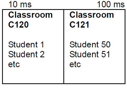
This experiment is a one-way
ANOVA design.
Why? Because each student was
bombarded with one beam.
We also say that this design is a
single-factor ANOVA.
Why?
Because each student was
bombarded with a single beam.
Another way of saying this is, that
each score in this experiment is
the result of one beam, one factor,
or one treatment. You may also
come across the term
one-way classification.
Now it will be easy for us to
understand two-way ANOVA.
An example of a two-way
ANOVA
A psychiatrist wanted to see
whether a combination of wine
and vitamin C may have an effect
on depression.
He randomly selected 10 male
patients, and also 10 female
patients, and randomly assigned
them in two groups: wine group, or
vitamin C group.
.
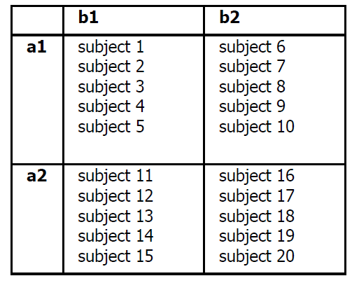
The layout of this experiment is
presented in the next table:
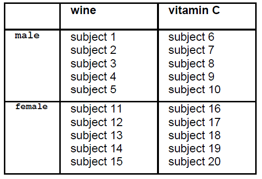
Look at subject 1. This subject is
influenced by two variables. Male
gender, and also wine. The score
of depression that he will give, will
be the result of these two factors.
For this reason, we call this type of
experiment a two-factor
experiment. The same, of course,
holds for all subjects. They are, in
a way, under crossfire. Two
factors hit them.
The layout above can also be
given in a more abstract form.
Variable A is gender, variable B is
nutrition. Each variable has two
levels, a1 a2 and b1 b2
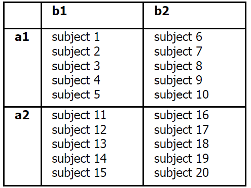
We say: We have two variables,
A and B. A is gender, B is nutrition.
Each of these two variables has
two levels. a1, a2, and b1, b2.
Because in this experiment we
use 2 variables with 2 levels each,
we call this experiment 2 x 2
factorial. We read this as follows:
two by two factorial.
The ANOVA summary table for
two-factor experiments is the
following:
ANOVA SUMMARY TABLE
Two-Way, 2x2 Factorial
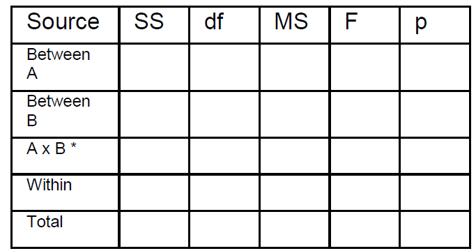
* Also called interaction
Things are getting complicated, I
hear you say.
I say: You already know everything
in this new ANOVA.
Our approach of understanding
the concepts and not memorizing
formulas has paid out.
Why do we have two Between
terms, A and B? you say.
Because here we have two
variables: gender, and nutrition,
i.e., A and B. We want to know if
gender (being male or female) has
an effect, and also if nutrition (wine
or vitamin C) has an effect.
Remember, the Between term is
the term that senses the effects of
our treatments.
The Within term we also know. It is
the variance of each group
separately. The sum of these
variances.
The Total term we also know. It is
simply the variance of all scores
without regard to what group they
came from.
The interaction term is a Between
term for cells taken diagonally:
mean for a1b1+a2b2 and mean
a1b2+a2b1. Look at the layout to
visualize this.
What is new here is the concept of
the interaction term. We need to
develop this concept, so we get a
gut feeling for it.
When you give two treatments to
subjects, one of the things you
want to see is whether the two
variables interact with each other.
To begin developing the concept
of interaction, let us consider a
simple experiment:
We give 5 mg of an anti-anxiety
drug, such as diazepam, and find
that this results in an increase in
the time patients sleep. This
increase is 2 hours.
Using different subjects, we find
that 200 ml of wine increase sleep
time by 1 hour.
Now if we give both 5 mg of
valium and 200 ml of wine, is it
sure that we will get 3 hours
increase in sleep time? Perhaps
yes, perhaps no. We know that
drugs may interact and produce
dramatic results, if given together.
You may have heard of cases in
which diazepam taken together
with alcohol caused coma, and
even death, because of
potentiation.
Students find the concept of
interaction difficult. For this reason
I will give an example later.
For the purposes of calculation of
this term in the ANOVA, there is no
problem. The df, as you would
expect, is the df of A x the df for B.
The SS you can calculate by
subtraction. SS total-(SS Between
A+SS Between B+SS within).
Alternatively, you can compute the
SS for AxB the same way you
calculated the between term, but
here calculate two means
diagonally, i.e.
mean for
a1b1+a2b2
and mean for
a2b1+a1b2.
Then we proceed with
the calculation of the variance of
these means.
The type of ANOVA design we are
discussing here is called factorial,
because in designing the
experiment we produce all
possible combinations.
In the above example we have:
Male - Wine, Male Vitamin C
Female - Wine, Female Vitamin C
Read this several times, it sounds
like a nursery rhyme. There is a
symmetry in it.
Visualizing the layout of
factorial designs
You will often come across
experiments that use these
designs, and if you go to graduate
school there is good chance you
will use them in your research.
We need to be able to visualize
the designs in order to understand
and evaluate them. A key
part of the task of a scientist is to
be able to critically evaluate the
research of others. Regrettably,
even reputable journals publish
research that is not sound.
We have considered so far a 2x2
design. How do we visualize this?
We see two characters (forget that
it is the number 2 here) separated
by the symbol x which stands for
times.
We have two things, two
variables, we therefore write down
A also B.
A B
Now we look again at 2x2 and this
time pay attention to what number
we have. Here we have 2.
We therefore write
A
a1 a2
Then we look at the number after
the x. It is also 2 (mind you it does
not have to always be 2, it can be,
4, 10 any number).
We therefore write
B
b1 b2
To sum up:
a1b1 a1b2
a2b1 a2b2
Read this several times, it sounds
like a nursery rhyme. There is a
symmetry in it.
This is how we visualize a 2x2
factorial:
a1b1 a1b2
a2b1 a2b2
Now let us consider this: 2x3 a1b2
a2a2b2
How do we visualize this? We
see two characters (forget that it is
the numbers 2 and 3 here)
separated by the symbol x which
stands for times. We have two
things, two variables, we therefore
write down A and also B.
A B
Now we look again at 2x3 and this
time pay attention to what
numbers we have. Before x we
have 2. We therefore write:
A
a1 a2
Then we look at the number after
the x. It is 3 (mind you, it does not
have to always be 3, it can be 4,
10, any number).
We therefore write:
B
b1 b2 b3
This is how we visualize a 2x3
factorial:
a1b1 a1b2 a1b3
a2b1 a2b2 a2b3
Now let us consider this: 2x3x5
How do we visualize this? We see
three characters (forget that it is
the numbers 2 and 3 and 5 here)
separated by the symbol x which
stands for times. We have three
things, three variables, we
therefore write down A, B,
also C.
A B C
Now we look again at 2x3x5 and
this time pay attention to what
numbers we have. Before x we
have 2.
We therefore write
A
a1 a2
Then we look at the number after
the x. It is 3 (mind you, it does not
have to always be 3, it can be, 4,
10, any number).
We therefore write
B
b1 b2 b3
Then we look at the third
number after the x. It is 5 (mind
you it does not have to always be
5, it can be, 6, 28, any number).
We therefore write
C
c1 c2 c3 c4 c5