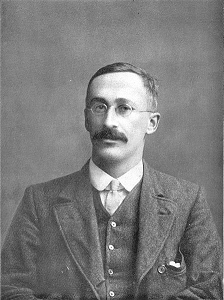
William Sealy Gosset
(June 13, 1876–October 16, 1937)
Wikipedia Aug, 2014 PD
William Sealy Gosset published
the t-test under the pen name
Student. We refer to the
distribution of this test as the
t-distribution. The t-test is a test of
inference, i.e., it allows us to infer
on the basis of our data, whether
the difference between two means
is reliable or, as we say, significant.
In what follows, we will first try to
develop the concepts needed for
understanding the logic and the
operations involved in the t-test.
We will talk about this and that and
the other. Be patient. Then we will
go over an example of the t-test.
Developing the concepts in the
t-test
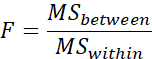
As is the case with all parametric
tests that we will cover in this
book, the t-test analysis is based
on variance.
In experiments in which we have
two groups we analyze our data by
using the t-test. There are two
types of t-tests. The t-test for
independent samples (groups),
and the other for dependent or
paired samples. Here we will
consider independent samples.
What are independent samples?
you say.
Ok. We will make a small
parenthesis in order to develop the
concept of independence.
Drama
Apple-pie IQ
A psychologist has a sneaky suspicion that
the type of apple pie has an effect on
intelligence. She randomly selected 20
students and randomly assigned them to
two groups. Group 1, golden delicious
apple pie, Group 2, red delicious apple pie.
John Gluck was assigned in Group 1, and
his friend Paul Crust was assigned to
Group 2. The psychologist proceeded with
giving these subjects a pound of apple pie
to eat. Subsequently she tested their
intelligence. Each subject was allowed to
see their intelligence score. There were 20
intelligence scores, one for each subject.
These groups are independent as you see.
She analyzed her data by using a t-test for
independent groups in order to see if there
was a significant difference in intelligence
in the two groups.
Note: An unexpected event occurred during the running of the experiment. One of the subjects in Group 2 did not show up on time so the experiment was delayed for a few minutes. John Gluck, who, as you remember, was in Group 1, offered to participate in Group 2, in addition to his participation in Group 1. The experimenter did not allow this. Had she allowed John Gluck to be a subject in both groups, she would have violated the rule of independence, and she would not have been able to analyze her data by using the t-test for independent samples.
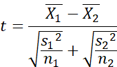
The formula for the t-test is:

We read this as follows:
T equals mean 1 minus mean 2
divided by the square root of the
variance of group 1 and group 2
divided by the number of scores
that went into the calculation of the
variance.
Faithful to our goal we must
understand the concepts in the
t-test.
First look at the numerator.
Mean 1 minus mean 2, that is the
difference of the two means.
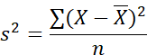
Next look at the denominator.
The square root of the variance
is the standard deviation.
This looks like the z formula that
we considered above. Here it is again:

Yes, you say, but the numerator of
the z formula is score minus the
mean. The numerator of the t-test
formula is mean 1 minus mean 2.
Where is the mean? They are not
the same, you say.
They are the same, I say. Mean 1
minus mean 2 is the difference
between the two means. Gosset
treats this difference as a score.
Yes, you say, but then where is
the mean in the t-formula?
The mean is there! I say.
It is there but you do not see it. It
is 0. The mean is zero.
Let the drums thunder at this
point. Let the bugles sound in the
four corners of the world!
The normal (t-) distribution with 0
in the middle. In other words, a
curve with a mean of 0.
A most important point in the history of
statistics.
Let us call this curve the
curve of no difference.
I do not understand the t formula
at the gut level, you say.
Watch the ritual dance with the
t-formula.
Drama
An archetypal ceremony II
I have a difference between
the two means. I hold this
difference up, wave it in the
air, I baptize it score. Then I
wear my glasses and stick my
nose on the t curve, running
up and down the line with
standard deviations on it, and
mumble: where does this
score fall? Where does this
score fall?
I then use the z formula -
oops, the t-formula - and
find where exactly our score -
oops, our difference - falls.
This is an archetypal ceremony.
Remember? Amazing, isn’t it? The
t-formula is actually the z formula!
I promised you that you do not
need the mind-boggling array of
fear inspiring formulas. Hang on.
Here is more of the story of the t
distribution. The motive in
Gosset’s mind was to modify the
normal curve so that it could safely
be used for small samples. He
decided to make it difficult for
researchers to find significance
(i.e., to decide whether the
difference between our two means
is reliable) when the samp
les are
small. The curve he created is a
normal curve with some intriguing
qualities. The noses, or tails of the
curve lift up as the sample size
decreases. The tails of the curve
lift up. You can see that in the graph that follows.
The shorter (lower) curve
corresponds to the smaller sample.
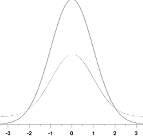
What an ingenious idea!
Some of you, few, very few,
already see what this means. It
means that it becomes more
difficult for you to find significance
because the percentage of the
curve increases in the tails so that
the magic standard deviation of
1.96 becomes larger, which in turn
makes it difficult for you to find
significance, that is to have a
“real” effect, a “true” finding so that
you can publish your experiment.
Let’s finish this story of the t-test,
a statistical test that is used so
frequently in labs across the world
daily.
So far, we have said that we have
two groups, therefore two means,
two standard deviations. We are
interested in deciding whether the
difference between the two means
is reliable, i.e., that it is not a
chance event, that it is, in a sense,
real. We find the t, which is
actually a z, that is, it tells us
where on the curve this difference
falls.
Ok, you say. So, we find the t
which is like z, then what?
If our sample is large the t
distribution is identical to the
normal distribution. In the normal
distribution, we have seen that z of
1.96 is an important mark.
Between -1.96 and +1.96 95% of
the curve falls. A score (here a
difference) that falls within these
two marking points, has a
probability of 95% to occur by
chance in a known situation in
which there is no difference, that is
in a situation in which the two
samples were drawn from the
same population. That is what our
curve of no difference graphs.
If our sample is small? you ask.
While in the normal distribution
1.96 always marks the 95% of the
curve, in the t distribution it is so
only if the sample size is very
large. With smaller samples, 1.96
increases inversely proportional to
sample size. The smaller the
sample size, the greater the
increase in 1.96.
Remember, again, Gosset’ s goal
was to make it difficult for
researchers to find significance
with small samples. He calculated
these new values of 1.96.
Drama
Mercy Mr. Gosset
Mr. Gosset, good morning. This is
Samir calling from India. I ran an
experiment with 20 subjects. How
much should I increase 1.96?
Half asleep, Gosset takes out his notes
and read the value to Samir.
The new value for z 1.96, the t, is
2.101.
Good night Mr. Samir.
Two hours later the phone rings again.
Good evening, Mr. Gosset. I am
Michel Duzed, calling from Montreal
Canada. Please give me the value of z
for an experiment with 72 subjects.
Gosset looks at his notes and says:
It is 1.994
Goodnight.
Going back to sleep is difficult for Mr. Gosset. One hour later the phone
rings again, this time from Japan.
Good day Mr. Gosset. Please give me
the new z for an experiment with 402
subjects.
1.966, Gosset says, and he hangs up.
I got to do something about this, he
says, aside from pulling the phone
from the plug. I got to do something…
I will never be able to sleep.
He did. He published his notes
with the recalculated z of 1.96.
Have you seen this in any
statistics book? All of my students
say no, actually a lot of my
colleagues say no, too. I will
disclose the secret. It is the
famous t-table found at the end of
every statistics book, including the
one you are reading now (see
Appendix). Promise to keep our secret between us.
Climax in the drama.
Samir of India wrote down the t
value:
2.101
With hands trembling he picked up
the sheet with the data analysis of
his thesis to find the result of the
t-test. He read it out aloud:
t=2.24
I made it! I made it!
he chants as he dances around in
his room. Samir will get his
Masters. The difference between
the two means of his experiment is
reliable.
He will report his finding as
significant. In his thesis he will
write:
This difference is significant
(p<0.05).
What does this notation mean?
It means that the chance that his
finding is not reliable, i.e., that it is a
chance event, is less than 5 per
cent.Scientists have agreed to accept
findings as being reliable if the p
value is less than 0.05.
Remember this!
Back in Canada Michel Duzed, holding the
note with the t value that Mr. Gosset just
gave her (it was 1.994, remember?),
compares it with the result of the t-test
value that she got by analyzing the data of
her experiment, which was t=1.982.
Alas! The t she computed by using the t
formula is smaller than the t Mr. Gosset
gave her.
Her eyes open wide, her face get gloomy,
and she collapses on an armchair. Michel
will not get her Doctorate. Her finding is
not significant. She will not write her
dissertation. If she were to write it, she
would report it as follows.
This finding is not significant (p>0.05).
P greater than 0.05.
This means that her difference could have
been a chance event more than 5 times in
a hundred.
Michel quits graduate school, she marries
her sweetheart and moves out of Quebec
to a job as a business consultant.
What happened to the Japanese
guy?
The curve of no difference, as we
said, has zero in the middle, that is
the mean is zero.
What does this curve graph?
Remember the curve in the case
of the woolen caps for the farmers
of the State of Wisconsin?
That curve was a curve
that we would be getting if we
were allowed to collect many
samples, figure out the mean of
each, and graph these means. In
effect this curve was empty.
But remember we knew
something about it. We knew the
estimate of the standard deviation
(standard error of the mean). We
calculated it from the standard
deviation of the one and only
sample mean we had.
In our present case, the t-curve is
a similar curve. It would be
graphing differences between two
means, if were we allowed to run
our experiment of two groups
many times, each time having two
means, calculating the mean of
each group and then calculating
the difference of the two means.
Because we have the standard
deviation of this curve, we can
consider our difference as a score
and engage in the ritual dance of
where my score falls. What point
on the standard deviation line
does this score (difference) lie.
We used the z formula to tell us
where on the curve our difference
lies. We said above that the
t-formula is actually a z formula, a
modified one, to take into account
the sample size. Let’s look at them
again.
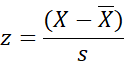
z equals score minus the mean
divided by the standard deviation.
t equals score (mean 1 minus
mean 2 gives us the difference
which we consider to be a score)
divided by the standard deviation
(the standard deviation of both
groups; remember that the square
root of variance is the standard
deviation).
You see then that the t is a z.
Why is the variance of each group
divided by the number of subjects
in the group?
Remember, Gosset’s goal was to
make it difficult to researchers to
find significance if their sample
size was small.
Understanding the logic of the
t-curve, the curve of no
difference.
Drama
Me minus me equals 1
Professor Lilly Prydum, a statistician,
decided to run a simple experiment to test
a model for guessing if two means came
from one specific group, or they came
from two different groups.
Quite convoluted, you say.
She invited Memy Tallibum, Ph.D. in
Education, to be part of the experiment
and try to guess if the difference of two
means came from the same group, or not.
The subjects were 30 students from
Trenton College. They were asked to take
a test of 120 questions on Chinese
geography, mythology, and culture. The
scoring of the test was done by a
computer, and the recording of the data
was done in such a way that the subjects
remained anonymous. The experiment
lasted 35 days. Subjects were asked not
to read about China during this time
period. They were also asked not to chat
amongst themselves and not to compare
notes.
Day 1 of the experiment. Time 9:00 in the
morning. The test is given. Time allotted 1
hour. 10:00 a.m. the testing period is
over. Students are asked to take a 30
minute break. During that time the exam
papers are graded, and the score is
recorded next to each subject. Dr.
Tallibum gets a copy of the results and
studies them with care.
At 10:30 the students are called back in
again, and are given the same test, the
one they took 30 minutes earlier. At
11:30 the testing session is over. The
subjects are thanked, and asked to be
back the next day. “Please be back here
at 9:00 in the morning sharp. And
remember, no reading on China”.
The students leave, their exam papers are
graded, and the score of each student is
recorded. Each subject now has two
scores. The score from session 1 and the
score from session 2. Dr. Tallibum gets a
copy and scrutinizes it. As expected the
difference between the first session and
the second is very small, and for most
students it is zero.
The next day all students are present, Dr.
Tallibum is present, and the experiment
proceeds as planned.
Session 1, the students are given the
same test they took the previous day. Session
2, the students are given the same test.
Scores are recorded and are handed to Dr.
Tallibum who watches like a hawk. At the
end of the second day Dr. Tallibum is not
surprised to see that, once again, the
difference between the first and the
second session is very small, close to zero.
Students are reminded that the
experiment will last 35 days, and asked to
“come back tomorrow “.
On day 16 of the experiment Dr. Tallibum
is surprised to see that the difference
between the first and the second session
is substantial. Students did not score as
well in the second session. The
explanation came in the evening as she
was watching the news. Pop star Mickey
Wiggletuchs had died. Students must have
heard about this during the break between
the two sessions and were emotionally
disturbed. That influenced their
performance in the second session.
On day 33 Dr. Tallibum was shocked to
see that the difference between session 1
and session 2 was so great. Scores in the
second session were so low! Again the
explanation came in the evening news.
The stock market had crashed. Apparently
the students heard of this disaster during
the break between the two sessions. Most
likely parents called and told their
children that there would be no money to
pay the college fees.
Day 34, the day before the last day
of the experiment, rolls smoothly.
At the end of the second session,
Dr. Tallibum is asked to leave the
exam room.
Students are given the same
instructions as usual. They are told
to be present as usual, for the last
day of the experiment.
Dr. Tallibum is left in the dark, she
does not know what the students
were told.
Day 35, the last day of the experiment.
Session 1. Students are taking the test
as in the past and Dr. Tallibum is
present, as in the past. During the
break the exam papers are graded and
scores handed to Dr. Tallibum.
At this point, there is a dramatic
change in the procedure. Dr. Tallibum
is asked to leave the exam room. She
is led to the elevator and taken to the
biology laboratories on the top floor,
where there are no windows. She is
asked not to leave this lab, not to
make any phone calls, and wait there
for an hour. To make sure, she is
guarded by the graduate students of
the biology lab.
At 11:30 the second session of the
experiment is over. The students are
told that the experiment came to an
end, that there was no need for them
to come back again, and were given a
brief talk as to the purpose of the
experiment.
The papers were graded, the scores
were recorded and Professor Lilly
Prydum, the experimenter, took the
elevator to the Biology Lab and
handed the results to Dr. Tallibum.
Dr. Tallibum, she said. In the second
session we prevented you from seeing
who were the subjects. As you realize
we may have used the same subjects,
the students from Trenton College, or
we may have used another group. We
could have used workers from the
Physical Plant of the College, students
from Trenton High, or senior citizens
from the local senior citizens club.
Your task is to guess whether the
group that took the test during today’s
second session of the experiment were
the Trenton College students that you
watched for 35 days, or another,
different group.
Dr. Tallibum looked at the data sheet. It
contained the difference between session
1 and session 2 for 35 days. The difference
score of day 35 was the score in question.
Instinctively, her eyes ran up and down
the list of differences. She was trying to
find if the score of day 35 has occurred in
the past 34 days. Not only that. If it has
occurred, how often has it occurred. If she
finds that it has occurred many times, she
will conclude that the students in the
second session of today were the same
students, that is the Trenton College
students.
If the difference score of today is not on
the list, if it has never occurred in the last
34 days, then the wisest guess would be
that in the second session of today it was
not the Trenton College students that took
the test.
It will be more difficult to guess if the
difference of day 35 has occurred a few
times, very few times. That's where Dr.
Tallibum will resort to her knowledge of
statistics. Guess what. She will draw
Goddess Normal Curve and pray. Let’s
listen to her reasoning out loud:
Dr. Tallibum’s soliloquy
The solution to my problem must be in the
normal curve, as always. What do I have
here. I have a difference between two
means but I do not know if the two means
came from the same group, or from two
different groups. I want to guess wisely. I
will start by placing 0 in the middle of the
normal curve. This is the curve of no
difference. I assume that this curve
graphs differences between means that
come from a known case, a case in which
all means come from the same group, the
same people. If the difference that I am
not sure about is 0 or close to 0, I can
safely conclude that this difference comes
from the same group of people, i.e., that in
both sessions of day 35 it was the Trenton
College students that took the test. If the
difference in question is large …ay, there's
the rub. Whether it safer to say same or
not say, and suffer the slings and arrows
of rough ridicule, or to shut up and by
going against my promise to participate,
my participation end. But behold, there is
light. I can compute the standard
deviation of this no-difference curve and
reason. I can engage in the archetypal
dance.
Behold Dr. Tallibum dancing around the
biology lab to the amazement of the bio
graduate students.
I have a difference between the two
means. I hold this difference up, wave it
in the air, I baptize it score. Then I wear
my glasses and stick my nose on the
normal curve, running up and down the
line with standard deviations on it, and
mumble: where does this score fall?
Where does this score fall?
I then use the z formula and find where
exactly my score - oops, our difference -
falls. If it falls within -1.96 and +1.96 then this score occurs frequently, 95% of the time, in this case of known no difference. If this score, difference, falls beyond 1.96 then it is a rare occurrence.
In this case the wisest guess is that it
does not come from the same group, that
is, in the second session it was not the
Trenton students but another different
group of people.
I hear a question. Speak up.
Can she find out what was this
new group, you say.
Yes, the Oracle of Delphi should
be able to tell you that.
Drama
The long jump
The prototypic experimenter is standing in
the middle of the normal curve holding his
score or difference in his hand. He is
focusing on 1.96 and is about to jump
beyond it. If he succeeds in jumping over
1.96, he gets a medallion (his degree
perhaps); if he does not succeed, he lands
on his behind, and gets a kick on the
same.
Talking seriously now. All statistical tests
are based on the same logic we developed
above. So, I advise you to read my
theatrical masterpieces carefully if you
want to get the concepts, and be able to
reason in statistics, and solve the
problems with only 5 formulas.
What are these 5 formulas?
The five formulas we need to know:

currently editing the formulas