

The layout of a 2x3 factorial ANOVA
In this example of a factorial design, we have a 2x3 (we read this as "a two by three") factorial. Two by three, meaning two factors: A and B. "two" meaning two levels for factor A. "three" meaning three levels for B. In another case of a 3x2 factorial design we have two factors, A and B, factor A three levels, factor B two levels.
FORMAT OF 2x3 FACTORIAL ANOVA SUMMARY TABLE
Interaction -factorial designs
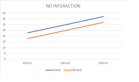
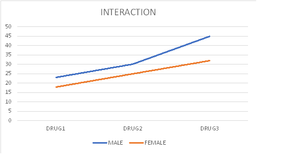
Note the term "Interaction" in the ANOVA summary table of the factorial design What is interaction? The best way to grasp the concept of interaction is to graph it.
ANOVA 2x3 factorial practice example
An experimenter wanted to test the effect of two drugs on the emotionality of male and female teenagers. He randomly selected 15 male and 15 female teenagers and randomly assigned them to 6 groups: Group 1, Group 2, Group 3, Group 4, Group 5, Group 6. five subjects in each group as shown in the following table.
The data are presented on the table below. The scores are the values recorded on a device measuring galvanic skin response, a measure of emotionality. Higher values indicate stronger emotion.
.
2x3 FACTORIAL ANOVA SUMMARY TABLE
After we calculate the F, we go to the F table to find the required F value for A, B, and AxB (interaction). Because,( remember?) the F ratio is A over within, B over within,
AxB over within, we enter the F table with
df of A and df within , which is 1 and 24.
also B and df within, which is 2 and 24
and lastly AxB within., which is 2 and 24. We first choose the F table at 0.05 level of significance.
Factor A: The F at df 1 and 24 is 4.25. In the summary table we see that the F for factor A (rows) is 62.31. This is greater than 4.25, so we conclude that here we have significance at the 0.05 level of significance; we say p<0.05, p less than 0.05. It has been accepted among scientists that at the 0.05 level we are allowed to say that we have significance, that the finding of our experiment is reliable.
Next we look at factor B. We enter the F table with df 2 and 24 and find F=3.50. This is less than the F of our summary table 502.19, therefore we conclude that we have significance at the 0.05 level. We formally express this as follows: p<0.05.
Next we look at AxB. We enter the F table with df 2 and 24 and find F=3.50.. This is greater than the F at the summary table value of 1.75 so we conclude that here we do not have significance. We formally express this as follows: p>0.05.
Step by step calculation of 2x3 ANOVA factorial
The goal of our calculations in ANOVA is to compute the F ratio, The F ratio is MS between over MS within. Mean Square is the mean of the squared deviations (differences).
of each score from the mean. These are very simple calculations involving high school mathematics. Simple as they are, they are very important concepts in data analysis and beyond, that is science in general. You will never need to perform these calculations. There are many free Statistics calculators online. However, for the purpose of developing the concepts of ANOVA here are the steps:
1. Calculate the mean of each group.
2. Subtract each score from the mean.
3. Square each difference
4. Add these squared differences. font red This is the Sum of Squares, the SS on the ANOVA summary table.)
5. calculate the degrees of freedom df (number of scores that went into the calculation of the mean minus 1)
6 Divide the SS by the df. Voila! this the MS.
7. The last step is to calculate the F. Divide MS by the MS of the error term (which is the MS within but may be something else depending on which ANOVA design you have. )
The F ratio, as all ratios, compares two things. For example the ratio 8/4 compares 8 to 4 and finds that 8 is two times greater than 4.