The z-table gives areas (probabilities) under the standard normal curve (mean $$\mu=0$$, SD $$\sigma=1$$).
Use it after you standardize a score:

Standardization (z-score):
$$z=\frac{x-\mu}{\sigma}$$
In words: $$z=\frac{\text{score} - \text{mean}}{\text{standard deviation}}$$

What the z-table shows

Most tables list the area to the left of a z value (cumulative probability).

• Left area at $$z=0$$ is 0.5000 (half the curve).
• Far left (negative big z) approaches 0; far right (positive big z) approaches 1.

Quick recipes

1) Probability below a score (left tail)
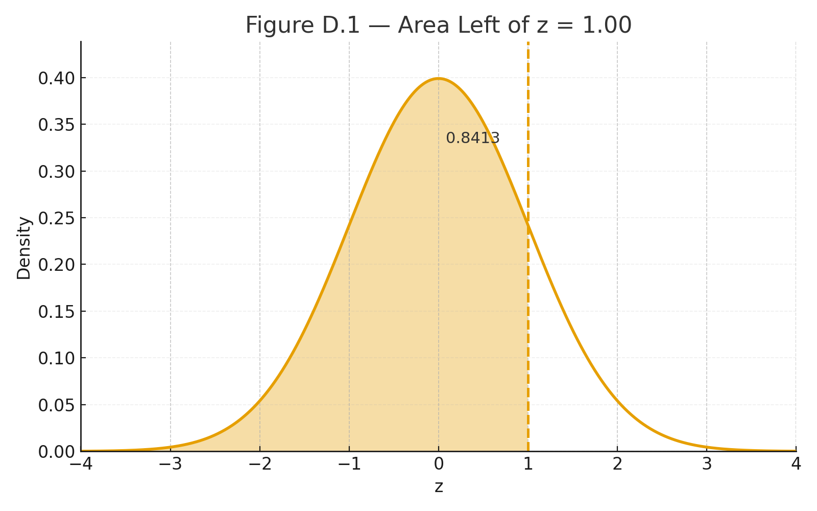
Example: $$z=1.00$$ → table gives 0.8413.
Interpretation: $$P(Z \le 1.00)=0.8413$$ (84.13% below).

2) Probability above a score (right tail)
Use complement: $$P(Z \ge z)=1-\text{left area}$$.
Example: $$z=1.00 \Rightarrow P(Z \ge 1.00)=1-0.8413=0.1587.$$

3) Probability between two scores
Subtract left areas.
Example: between $$z= -0.50$$ (left area 0.3085) and $$z=1.20$$ (0.8849):
$$P(-0.50 \le Z \le 1.20)=0.8849-0.3085=0.5764.$$

4) From a raw score to probability
Test scores: $$\mu=100, \ \sigma=15$$. What % are below 115?
Standardize: $$z=\frac{115-100}{15}=1.00 \Rightarrow 0.8413 \ (\text{84.13%}).$$

5) From probability to raw score (percentile)
What score is the 90th percentile?
Find z with left area ≈ 0.9000 → $$z \approx 1.2816$$.
Convert back: $$x=\mu+z\sigma=100+(1.2816)(15)=119.22.$$

Tips

• For negative z, use the table’s symmetry: left area at $$-z$$ equals 1 − left area at $$+z$$.
• Rounding: two decimals is common (e.g., 1.23).
• Modern tools (calculator/Sheets/Python) can give exact p-values directly.

Visuals

Figure D.1 — Normal curve with area left of z = 1.00 shaded (0.8413).
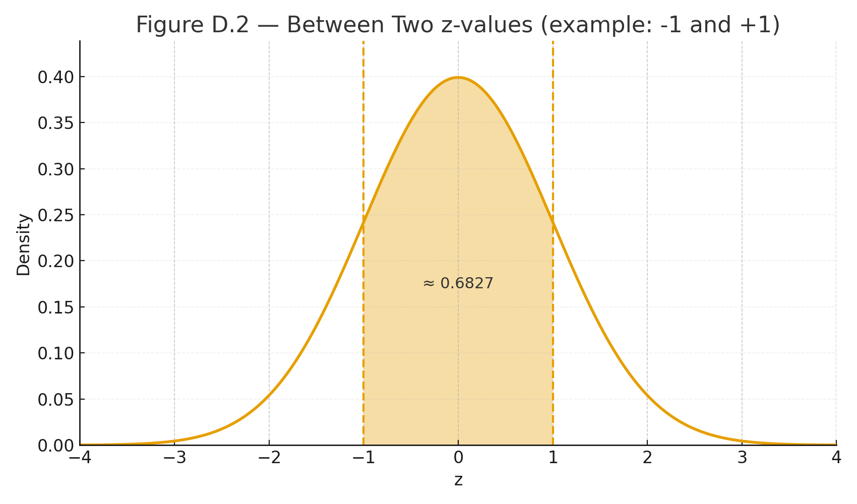
Figure D.2 — Two-z shaded band for “between” probability.

📱 QR: Online z-calculator (type z or x, get areas instantly)

Practice self-test quiz

In the space below, please find practice problems and self-test quizzes. For full access, please signup free.

Tables give the critical values we compare our test statistic against.
They depend on:

• The significance level (α, often 0.05)
• The degrees of freedom (df)

t-table

• Rows = degrees of freedom (df)
• Columns = significance level (α)

Example:

• Independent-samples t-test with n₁ = 12, n₂ = 12
• df = 12 + 12 – 2 = 22
• At α = 0.05 (two-tailed) → critical t ≈ 2.07
• If $$|t| \geq 2.07$$ → significant

F-table

• Needs two df values:
  • df between (numerator)
  • df within (denominator)

Example:

• One-way ANOVA, 3 groups, N = 24
• df between = k – 1 = 2
• df within = N – k = 21
• At α = 0.05 → critical F ≈ 3.47
• If computed F ≥ 3.47 → significant

Student Tips

• Always compute df correctly.
• Use tables if no software is available.
• Most calculators or apps today give exact p-values — faster than tables.

📱 QR: Interactive critical value calculator (t and F tables online)

Visuals

Figure C.1 — Snippet of a t-table row (df = 22, α = 0.05 highlighted).
Figure C.2 — F-table grid with numerator df = 2, denominator df = 21 marked.

Practice self-test quiz

In the space below, please find practice problems and self-test quizzes. For full access, please signup free.

A quick refresher on the math you’ll need in this book.

Order of Operations (PEMDAS)

• Parentheses → Exponents → Multiplication/Division → Addition/Subtraction
• Example:
  $$3 + 2 \times (4^2) = 3 + 2 \times 16 = 35$$

Fractions and Division

• Example:
  $$\frac{24}{6} = 4$$

Square Roots

• Example:
  $$\sqrt{9} = 3$$
• Example:
  $$\sqrt{\frac{16}{4}} = \sqrt{4} = 2$$

Summation Notation (Σ)

• Means “add them up.”
• Example:
  $$\Sigma X = 2+5+7 = 14$$
• Example:
  $$\Sigma (X-\bar{X})^2 = (2-4)^2 + (5-4)^2 + (7-4)^2 = 4+1+9 = 14$$

Exponents and Squares

• $$x^2 = x \times x$$
• Example:
  $$5^2 = 25$$

Mini Example: Variance and Standard Deviation

Data: 6, 8, 10

1. Mean:
   $$\bar{X} = \frac{6+8+10}{3} = 8$$
2. Deviations: –2, 0, +2
3. Squared deviations: 4, 0, 4
4. Variance:
   $$\frac{8}{2} = 4$$
5. Standard deviation:
   $$\sqrt{4} = 2$$

📱 QR: Algebra refresher video (scan for a quick math warm-up)

Practice self-test quiz

In the space below, please find practice problems and self-test quizzes. For full access, please signup free.

Welcome to Part 8 — Appendices of this free online high school statistics textbook. This essential reference section provides quick-access cheat sheets, reviews, statistical tables, technology tips, and supporting resources to help you throughout the course. From symbols and notation to probability tables, math refreshers, practice datasets, study strategies, and a comprehensive glossary, these appendices are designed as reliable tools for high school students, AP Statistics preparation, and anyone needing clear statistical references.

Perfect for quick lookups during homework, exam review, or practical applications, Part 8 complements the main lessons with statistical tables, formula references, technology guidance, and study support—all presented in a clear, accessible format to build confidence in descriptive and inferential statistics.

Appendices in Part 8

1. Appendix 1 — Symbols and Notation (Cheat Sheet) – Quick reference for common statistical symbols, Greek letters, and notation used throughout the book.
2. Appendix 2 — Math Review for Statistics – Review of essential algebra, summation notation, and foundational math skills needed for statistics.
3. Appendix 3 — Using the t-table and F-table – Guidance on reading and applying t and F distribution tables for hypothesis testing.
4. Appendix 4 — Using the z-table – Step-by-step instructions for the standard normal (z) table and probability calculations.
5. Appendix 5 — Technology Tips (On Your Phone & Laptop) – Practical guidance for calculators, spreadsheets, statistical software, and mobile tools.
6. Appendix 6 — Data Sets for Practice – Real and simulated datasets for hands-on learning and concept reinforcement.
7. Appendix 7 — Study Tips for Statistics – Effective strategies for learning, reviewing, and succeeding in statistics courses.
8. Appendix 8 — Glossary of Key Terms – Clear definitions of essential statistical vocabulary from descriptive through inferential statistics.
9. Appendix 9 — The Normal Distribution Table – The standard normal (z) table for probability lookup and interpretation.
10. Appendix 10 — The t table – Critical values of the t distribution for confidence intervals and hypothesis tests.
11. Appendix 11 — The F-table – F distribution tables used in ANOVA and variance-based hypothesis testing.

These appendices are designed to function as quick-reference tools you can return to again and again. Use them for checking symbols, reviewing formulas, consulting probability tables, reinforcing concepts, and supporting your work across the entire statistics course.

A quick reference to the symbols used in this book.

Practice self-test quiz

In the space below, please find practice problems and self-test quizzes. For full access, please signup free.

Modern statistics and AI are powerful.
They analyze millions of records, make predictions, and even guide decisions.
But with this power come ethical responsibilities.

Bias in Algorithms

Algorithms learn from data.
If the data are biased, the algorithm will repeat — or even amplify — the bias.

Example:

• If past hiring data favored men, an AI trained on it may also favor men.

Lesson: Always ask, whose data are we using, and what history do they reflect?

Privacy and Data Use

Big data often comes from personal information: browsing, phones, sensors.
Students, patients, and citizens deserve protection.

• Informed consent
• Secure storage
• Respect for anonymity

Transparency and Accountability

AI systems are sometimes black boxes.
Users may not know how a decision was made.

Ethical practice means:

• Explaining decisions in plain language
• Allowing appeals and corrections
• Sharing responsibility between humans and machines

Example: Predictive Policing

• Data show more arrests in certain neighborhoods
• AI predicts more crime there → police increase presence
• Result: cycle reinforces itself

This shows why ethical reflection is essential.

Guiding Principles

• Fairness: avoid discrimination
• Privacy: protect individual rights
• Transparency: explain decisions
• Accountability: humans must remain responsible

Visuals

Figure 19.1 — Ethics Triangle: Fairness, Privacy, Transparency at the three corners.

Why This Matters

Statistics and AI are not only technical.
They are also social, cultural, and ethical.
Future scientists, teachers, and citizens must understand both the power and the responsibility of data.

Practice self-test quiz

In the space below, please find practice problems and self-test quizzes. For full access, please signup free.

Artificial Intelligence (AI) aims to build systems that can learn, adapt, and make decisions.
One powerful tool is the neural network, inspired by the brain.

From Statistics to AI

• Regression predicts Y from X
• Logistic regression predicts probability (0–1)
• Neural networks generalize this idea: many inputs, many layers, nonlinear patterns

The Structure of a Neural Network

1. Input layer — variables (X₁, X₂, …)
2. Hidden layers — units that transform the input
3. Output layer — prediction or classification

Each connection has a weight (like a slope in regression).

Formula for a Neuron

A single unit in the network:

$$z = \sum w_i X_i + b$$

$$y = f(z)$$

Where:

• $$w_i$$ = weights
• $$X_i$$ = inputs
• $$b$$ = bias (like an intercept)
• $$f(z)$$ = activation function (e.g., logistic, ReLU)

Learning in a Network

The network predicts outputs and compares them with the true answers.
The error is sent backward through the network to adjust weights.
This is called backpropagation.

Example

Predicting if a student will pass or fail based on:

• Study hours
• Attendance
• Practice problems completed

Inputs → combined with weights → logistic activation → output: probability of passing.

Visuals

Figure 18.1 — Simple Neural Network (Inputs → Hidden → Output)

Figure 18.2 — Activation Functions

Why This Matters

• Neural networks extend regression and logistic regression.
• They allow learning from large, complex datasets (images, speech, language).
• Modern AI (translation, recognition, chatbots) is powered by these models.

Practice self-test quiz

In the space below, please find practice problems and self-test quizzes. For full access, please signup free.

Simple regression predicts Y from one X.
But in real life, outcomes often depend on several variables — or may not be linear.

This chapter introduces multiple regression and logistic regression.

Multiple Regression

Formula:

$$\hat{Y} = a + b_1X_1 + b_2X_2 + \dots + b_kX_k$$

In words:
$$\text{Predicted Y} = \text{intercept} + (b_1 \times X_1) + (b_2 \times X_2) + \dots$$

Where:

• $$X_1, X_2, \dots X_k$$ = predictors
• $$b_1, b_2, \dots b_k$$ = slopes (weights for each predictor)

Example: Predicting college GPA from:

• High school GPA ($$X_1$$)
• Study hours ($$X_2$$)

Equation:
$$\hat{Y} = 1.0 + 0.5X_1 + 0.1X_2$$

Interpretation:

• For each 1-point increase in HS GPA, college GPA rises 0.5.
• For each extra study hour, GPA rises 0.1.

Coefficient of Determination

In multiple regression, $$R^2$$ tells us the proportion of variance explained by all predictors together.

Example: $$R^2 = 0.65$$ → predictors explain 65% of the outcome’s variability.

Logistic Regression

What if the outcome is yes/no (categorical)?
Example: Will a student pass or fail?

We use logistic regression.

Formula:

$$P(Y=1) = \frac{1}{1 + e^{-(a + bX)}}$$

In words:
$$\text{Probability of success} = \frac{1}{1 + e^{-(\text{intercept} + \text{slope} \times X)}}$$

Output: probability between 0 and 1.

Example: Predicting pass/fail from study hours.

• Equation: $$P = \frac{1}{1 + e^{-( -2 + 0.5X )}}$$
• If X = 6 hours: $$P = \frac{1}{1 + e^{-1}} = 0.73$$
• About 73% chance of passing.

Visuals

Figure 17.1 — Multiple regression plane: Y predicted from two predictors.

Figure 17.2 — Logistic regression curve: probability vs. study hours.

Why This Matters

• Multiple regression = prediction with many factors
• Logistic regression = prediction when the outcome is categorical
• $$R^2$$ = strength of prediction

These methods expand the power of regression beyond a straight line, preparing for modern predictive modeling.

Practice self-test quiz

In the space below, please find practice problems and self-test quizzes. For full access, please signup free.

Machine learning is where statistics meets computers.
Instead of only writing formulas, we teach a computer to learn patterns from data.

What is Machine Learning?

Machine learning uses algorithms to improve automatically with experience.

• Supervised learning: the computer is given examples with correct answers.
• Unsupervised learning: the computer finds patterns without answers.

Supervised Learning

Goal: predict Y from X.

Examples:

• Predict exam scores from study hours
• Predict house price from size, location, and age

Steps:

1. Split data into training set and test set
2. Train the model on training data
3. Test accuracy on new (unseen) data

Formula (simple linear regression as machine learning):
$$\hat{Y} = a + bX$$

Here, the computer “learns” $$a$$ and $$b$$ from the data.

Unsupervised Learning

Goal: find hidden structure in the data.

Examples:

• Group students by study habits
• Cluster shoppers by buying patterns

Algorithms:

• k-means clustering
• Hierarchical clustering

No “correct answer” is given — the computer organizes the data.

Overfitting vs. Generalization

• Overfitting: the model memorizes the training data but fails on new data.
• Generalization: the model captures the underlying pattern and works on new data.

Example:
If a student memorizes past exam answers (overfit), they may fail a new test.
If they learn the concepts (generalize), they succeed.

Key Concepts

• Training set: data used to build the model
• Test set: data used to evaluate performance
• Accuracy: how well the model predicts new data

Visuals

Figure 16.1 — Supervised learning example: regression line predicting Y from X.

Figure 16.2 — Unsupervised learning example: scatterplot with clusters (k-means).

Figure 16.3 — Overfitting vs. generalization: wiggly curve vs. smooth line.

Why This Matters

Machine learning grows directly out of statistics:

• Regression → prediction
• ANOVA → group classification
• Clustering → organizing data

By learning the basics of ML, students see how statistics powers AI.

Practice self-test quiz

In the space below, please find practice problems and self-test quizzes. For full access, please signup free.

Classical statistics uses formulas and tables.
Modern computing gives us another way: resampling and simulation.

Instead of relying only on theory, we let the computer generate thousands of samples and see what happens.

Bootstrapping

Bootstrapping means resampling with replacement from the original data.

Steps:

1. Take a sample of size $$n$$ from the data (with replacement).
2. Compute the statistic (mean, median, correlation).
3. Repeat thousands of times.
4. Use the distribution of resampled statistics to estimate confidence intervals.

Example:
Data = [5, 6, 7, 9].
Resample 1000 times, compute mean each time.
The distribution of means gives an estimate of the true mean’s variability.

Randomization (Permutation) Tests

Used to test hypotheses by shuffling labels.

Steps:

1. Combine all data.
2. Randomly assign to groups.
3. Compute the difference in means.
4. Repeat thousands of times.
5. Compare the observed difference to this distribution.

This shows whether the observed effect could be due to chance.

Monte Carlo Simulation

Monte Carlo methods use random numbers to model complex processes.

Example: Estimating $$\pi$$.

• Randomly throw points into a square.
• Count how many fall inside the circle quarter.
• $$\pi \approx 4 \times \tfrac{\text{inside circle}}{\text{total points}}$$.

Why Resampling Works

Resampling uses the data itself as a model of the population.
It avoids assumptions (like normality) and adapts to modern computing power.

Visuals

Figure 15.1 — Bootstrapping illustration: resampling from a small dataset with replacement.

Figure 15.2 — Randomization test: labels shuffled between groups.

Figure 15.3 — Monte Carlo: random points filling a square and a quarter circle.

Why This Matters

Resampling and simulation show students that statistics is not only about formulas.
Computers allow us to see probability in action.
This approach prepares students for data science, where simulation is as important as theory.

Practice self-test quiz

In the space below, please find practice problems and self-test quizzes. For full access, please signup free.