Story 15 — Analysis of variance One-way ANOVA
Analysis of variance is used by
scientists in order to analyze data
from experiments of literally
unlimited experimental designs. It
is most popular and dominant
statistical test in the biological and
social sciences. The complexity of
these designs ranges from very
simple to frighteningly convoluted.
The formulas are so many that no
statistical book contains all of
them.
As I promised you, we will
navigate through this ocean with
no formulas. We do not need
them. If we understand what we
are doing, if we get the concepts
involved, we do not need
formulas. Do you need a map in
order to work around your
kitchen?
Hurray, here we launch the big
ocean liner, ANOVA!
What is ANOVA, what do we do in
Analysis of Variance?
We analyze variance.
That is tautologous, you say.
Ok, we partition the variance. That
is pretty much what we do.
Variance I know well, you say.
Analysis of Variance you know
pretty well, I say.
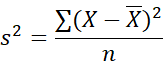
Yes. Variance we know so well.

Remember? The sum of squared
deviations of each score from the
mean, and all of this divided by n,
the number of scores that went
into the calculation, i.e., here, the
number of all scores.
Why do you say “here”, you ask.
Good observation. n does not
always represent the number of
scores in an experiment. It is the
number of observations, that is a
safer way to say this. More of that
soon. I was saying that what we do in
ANOVA is analyze the variance in
our data, more specifically, we
partition the variance.
What is the result of this analysis?
Is it a t?
Something like a t. A modified t, I
would say.
You said earlier that it is a modified z.
You are very observant. Yes. As I
told you earlier, statistics is like a
pyramid. Discoveries are based
on earlier discoveries.
There is continuity. If you brush
aside the many formulas and
concentrate on concepts, you get
a marvelous view of the edifice of
statistics. Then you are in
command. You can take decisions,
be in a position to critically view
experiments, defend yourself
against criticism that is thrown at
you, and ultimately add this
knowledge to your personal
philosophy.
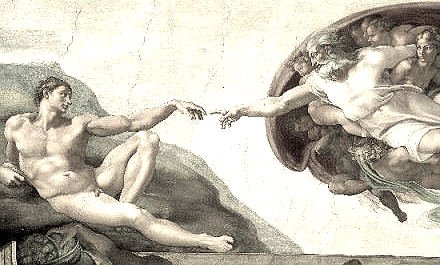
Drama
Clip his tail
Fisher was determined to clip Gosset ‘s tail
a bit.
That Gosset, he thinks he is smart. He
rides high in the world with his stupid
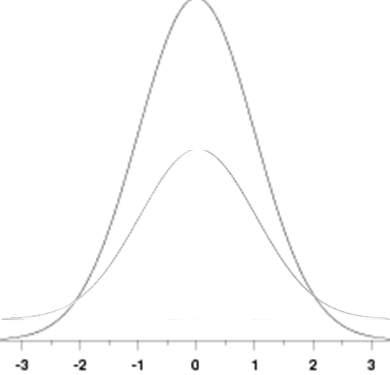
t-distribution. Big deal! All he did was to
add one puny column on the left of the
normal distribution. The df column. Oh,
yes, ok, ok…He did recalculate the z, big
deal.
Fisher had been scratching his head for
months, engaging in obsessive dialogues
with Gosset, downgrading his achievement
but deep down he knew he was jealous.
I got to come up with something myself.
What if I add another column to the
normal distribution. Another column of
what? Not df again? If not df, what then.
I got to be more original. How about
another line on top of the t table.
He did. The df Between.
Good Knighthood, Sir Fisher.
The result, the endpoint of
ANOVA, is F. This is in honoring
Fisher who developed ANOVA.
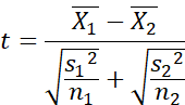
We calculate the F by the so
called F ratio which is:

We read this as follows:
F equals mean square between,
divided by mean square within.
Remember that mean square is
another way of saying variance.
So, you should not be worried with
the F ratio.
What about between and within?
you say.
That is easy. In computing the
variance between we calculate a
variance. We line up the means of
the various groups in our
experiment, we treat them like
scores, and figure out the
variance.
You are kidding, you say. I have
seen terrifying formulas for even
the simplest ANOVA.
You are correct.
Now the second part of your
question. Mean square within.
Easy again. You already know it.
We compute the variance of the
first group, and write it down, then
we compute the variance of the
second group and write it down,
then we do the same for all the
groups in our experiment. The
number of groups can vary from 2
to as many as you wish. In the end
we simply add these variances.
That gives the variance within.
Amazing! you say. No new
formulas for ANOVA!
You can use ANOVA right away. All
you needed was to get the concepts of variance between and
variance within.
What about partitioning the
variance? you say.
Variance between and variance
within, if added together, give us
the Total variance.
Total variance can be computed if
you calculate the variance of all
the scores of all your groups,
disregarding what group a score
came from. Again, all you need is
the familiar variance formula.
That is unbelievable, you say. I am
confused. Every statistics book
gives ANOVA summary tables.
Yes indeed. That is the
convention, but it is not necessary
in order to compute the F ratio. In
practically every case in which
step by step instructions are given
(without first developing the
concepts) things acquire an aura
of awesome complexity and
difficulty, and, I am afraid, fake
importance.
Because you and I cannot go
against the whole world, let’s take
a quick look at the typical
presentation of ANOVA. Up until
the sixties, journals were including
ANOVA summary tables in the
publications. As I said, this gives a
publication the semblance of
quantitative science, but, alas,
at times only a semblance.
ANOVA SUMMARY TABLE
One-way ANOVA
We know every term on this table.
Within is also called the error term.
The error term is the term which
goes in the denominator of the F
ratio. In more complex designs,
the error term may be other than the
within term.
Review the five formulas that are
needed for virtually all parametric
statistics. Do not simply memorize
them, look into them conceptually


An example of ANOVA
A biologist wanted to see if
quantity of vitamin C in diet may
reduce body weight. He randomly
selected 15 male rats and
randomly assigned them to the
following three groups. Group1 10
mg, Group2 20 mg, and Group3
30 mg. He added this vitamin in
the food of the rats daily for 30
days. On the 30th day he weighed
the rats.
Here are the data and the
ANOVA table.
ANOVA SUMMARY TABLE
One-way ANOVA
The analysis showed that we have
a significant effect. The differences
between the means are
significant, i.e., reliable. The p
value is less than 1 in 10000. This
means that the probability that the
difference we report is a chance
event (and not the result of our
treatment of giving rats vitamin C)
is less than 1 in 10000.
How did you compute the degrees
of freedom, df, you ask.
You know this if you know the
concepts of Between, Within, and
Total.
We said, in order to compute the
variance between, we line up the
means of all the groups and treat
them as scores, and calculate the
variance. How many means we
have here? We have three means.
We really consider them as scores
here. In order to calculate the
variance of three numbers, we
must first calculate the mean. By
calculating the mean, we lose 1
degree of freedom for every mean,
remember? So, our df for the
between term is 3-1=2.
We calculate variance within as
we said above. We calculate the
mean of the first group and then
the variance of this group. Then
we do the same for the second
group, and then the third group.
We add these 3 variances and this
gives us the variance within. Since
we compute 3 means in the
process of calculating the
variances, we lose 3 degrees of
freedom. How many scores went
into the calculations of variance
within? All the sores, that is 15.
Our degrees of freedom then are
df=15-3=12.
Easy, no formulas needed,
because we understand the
concept of df and also variance
within.
Lastly, we compute the df of Total
as follows:
In order to compute the Total
variance, we said, we take all of
the scores of all the groups
disregarding what group each
score comes from. In order to
calculate this variance we must
first calculate the mean, therefore
we lose 1 degree of freedom. How
many scores went into the
calculation of the Total variance?
All of the scores, here 15. Our
degrees of freedom for Total then
is 15-1=14.
Note that adding up the df for
Between and Within we find the df
for Total.
That is what we meant by
partitioning. We said we partition
variance.
Here we partition the Total
variance into variance
between and variance within.
Indeed, verify that SS between
plus SS within equals SS Total.
That is,
1259 + 373.2 = 1632.2
How did we get the p value? you
ask.
I will be very practical here. As
was the case with the t-distribution,
here too, there is a table with the F
values (see Appendix).
These are in a way the recalculated
1.96, that is the point on the curve
beyond which 5% of the curve lies.
In the case of the t curve we
entered the table with the degrees
of freedom and found the required
t at the 5% level. In the present
case, we enter the F table with the
degrees of freedom for Between
(in the present experiment df=2)
and the degrees of freedom
for Within (in the present
experiment df=12). We locate the
F on the table. This is the required
F.
Then we compare the obtained F
(the one we calculated, look at he
summary table) to the required F.
As in the case of the t-test, if our
obtained F is greater than the
required F, we have significance.
We then say p<0.05.
I understand how we calculate df
without formulas, however I do not
see why we need it.
I see why you are confused. As I
said this is what happens every
time we try to teach in a
mechanistic, compulsive, step by
step way. The general practice of
working with formulas blindly, and
using the ANOVA summary table,
often prevents the student from
seeing what is going on.
As I said at the beginning, the
ANOVA summary table is not
needed. What you need to do is
simply calculate the variance, and
compare the variances, that is the
F ratio. df is simply the n in the
variance formula.
I understand variance Between,
variance Within, and df.
However, I do not see why the F
ratio can detect significance, you
say.
A very important question, if
indeed, we are sincere when we
say we want to understand the
concepts and the logic of statistics.
Drama
Master of the waves
It is a beautiful, cool, calm day in
Puerto Rico. You are sitting in a San
Juan small café, nested on the rocks
overlooking the magnificent Atlantic
ocean. You are happy, sipping your
coffee, Bacardi on the side, and slowly
nibbling on a sinfully sweet piece of PR
cake. It is quiet, the only thing you
hear is the rhythmic sound of waves
gently breaking on the foundations of
the cafe. Suddenly you hear voices; it
sounds like people are arguing. Soon
their voices become loud enough, you
can clearly hear what they are saying.
You don’t believe me? Look again.
See? I caused that wave.
There is much laughter.
Buddy, you are nuts, that’s what I
say. The only waves you cause is in
your brain. You go and see a shrink!
The argument grows in intensity and
the guy with the claims to
supernatural powers, keeps throwing
small stones into the sea. You decide
to join the noisy group and get the
argument straight.
Guys, I have the answer to your
argument. I will show you who is
right. For now, let the sea rest and
calm down, just in case this guy has
disturbed it. Come sit and have a cup
of coffee.
Ten minutes later, you take the lot to the edge of the rocks.
First, we will measure the heights of the next 40 waves and record these data, you say.
When forty waves have been recorded, you
turn to the guy with the supernatural claims
and say:
Ok, this is your show now.
The guy, his confidence somewhat deflated,
picks up a stone and hurls it into the sea. All
eyes are fixed on the base of the rock, waiting for the next wave. The wave comes and is recorded.
The moment of truth, you say.
The height of the wave is read out loud. It is
not taller than any of the 40 waves previously recorded. The miracle worker receives a truckload of cosmetic epithets and soon the café slips back into the beatific serenity. Sleep hovers over your eyelids. You dream of conquistadors and
fierce Carib Indians, of rituals and dances that humans created in an attempt to understand their world.
Cute story, but I still do not
understand why the F ratio can
indeed measure that we have
significance, you say.
The forty waves provided us with
what I call the “endogenous”
variance, baseline, the variation in
the heights of the waves that is
present when no obvious cause
can be seen. The wave after the
action of the ambitious miracle
worker was the presumed effect of
his manipulation (in statistics we
call this treatment). Comparing the
baseline with the claimed effect of
his manipulation can give us
support, or lack thereof, for a
connection between what he did
and the result we observed.
If the result which he claims that
he caused by his manipulation is
bigger than the natural,
(endogenous or spontaneous
variance), then we may say that
he caused the effect by his
manipulation.
A brief parenthesis at this point to make
sure we understand what we mean by
saying ratio. Alas, mechanistic methods
of teaching arithmetic without
development of concepts, often prevent
the pupil from understanding that in
division, what we do is compare two
numbers: the numerator to the
denominator. If you have 20 dollars, and
I have 5 dollars, in dividing 20 by 5, I
compare 20 to 5. You have 4 times
more money than I have.
Our treatment causes variance
between to increase? you say.
Yes, let’s see it in an example.
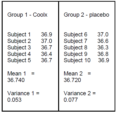
A pharmacologist is testing a new
drug (tentatively named Coolx)
that is suspected to lower body
temperature. He randomly
selects 10 male college students
and randomly assigns them to
two groups. Group 1 receives
Coolx, Group 2 receives a
placebo (an inert substance that
has no effect on physiology).
Here is the layout of the
experiment.
Before the experiment proper, the
pharmacologist records the
temperature of the subjects, in
order to have the baseline
temperature, the temperature that
is present without any
manipulation on the part of
the experimenter.
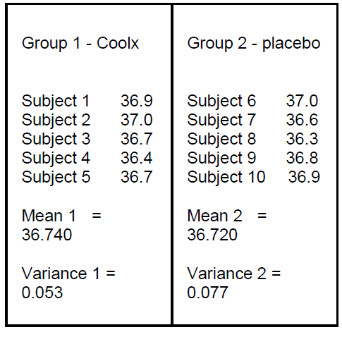
Here is the baseline temperature
(Celsius)
We will now calculate variance
between.
Remember, in order to calculate
variance between we line up the
means and treat them as scores.
We then proceed and calculate the
variance of these scores.
Here we have two means
36.740 36.720
The variance of these two scores
is 0.053. This is variance between.
The next table shows temperature
after the administration of drug
Coolx to Group 1
Note that the mean in Group 1
decreased. It was 36.740 before
giving the drug, it is 35.94 now.
Also note that the variance of this
group did not change.
Now the big moment has arrived.
Has the variance between
changed? If yes, we will be
convinced that variance between
is sensitive to our manipulation,
i.e., that it senses the effect of the
drug.
As usual, in order to calculate
variance between, we line up the
means and treat them as scores.
We then calculate the variance of
these scores.
The means here are:
35.94 36.720
The variance is 0.3042.
This is variance between.
Let’s compare this to variance
between before our manipulation
of giving the drug:
We saw above that variance was
0.053 .
Voila! After giving the drug, that is
after our treatment, variance
between changed. Variance within
did not change.
Conclusion: The F ratio is
sensitive to our treatment. It does
so, because variance Between
changes because of our
manipulation, while variance
Within does not change.
Why? you say.
Remember that variance
measures the distance of scores
from the mean. The mean can
increase or decrease but the
distance of scores from the mean
does not change. The scores
move up or down with the mean.