
Statistics 2nd ed


Story 18 — Complex, mixed, split-plot designs ANOVA
In this story we will develop the concept of mixed designs and give a practice example.
Elegant research avoids complex
designs also called split-plot designs
or mixed designs. However, you may not
be spared of these monsters in your
student or research life.
Let’s get a whiff of these monsters.
A psychiatrist wanted to see, if two
new drugs improve the condition
of depressive and schizophrenic
patients.
He randomly assigned 4
depressive patients to Drug1 and
Drug2 conditions. That is, each of
the depressive patients will be
serving as a subject in both the
Drug conditions. This is a repeated
measures design.
He did the same with the
schizophrenic patients. He
randomly assign 4 schizophrenic
patients to Drug1 and Drug2
conditions. That is, each of the
schizophrenic patients will be
serving as a subject in both the
Drug conditions. This is a repeated
measures design.
As you see, here we have two
independent groups (depressive
patients, and schizophrenic
patients) but each patient is given
two treatments, that is he is tested
repeatedly, i.e., in both drug
conditions. We have a hybrid
situation, you would say. Both
independence and non-
independence in the same
experiment.
Here is the layout; X stands for scores.
The analysis of data in complex
designs like the above, is, as
always, an operation involving the
calculation of variance. The
interpretation of the results of such
an analysis is like the interpretations
we considered in this book so far.
ANOVA mixed split plot - formula and practice example
What is ANOVA mixed split plot design
ANOVA mixed split plot designs are complex designs that employ both independent and repeated measures. The best way to explain this is to present the layout of these experimental designs.
TABLE SHOWING THE LAYOUT
OF MIXED SPLIT-PLOT DESIGNS
Observe that there are two independent groups, depressive, and schizophrenic. Also observe that each subject of the depressive and schizophrenic groups is repeatedly tested, once with Drug 1, and later with Drug 2. This is a repeated measures arrangement So here we have a design in which independent and repeated measures are mixed. The name split plot comes from the fact that this design is extensively used in agricultural research.
ANOVA mixed split plot designs formula
As in all ANOVA, the formula for these designs is:

We read this as follows: Mean square between over mean square within. What is mean square, you ask? It is the mean of squares. What is squares, you ask. Squares is the statistical term for squared deviations (of squared differences) of each score X from the mean. What are the squared differences, you ask. Remember the formula for variance?

Look at the numerator
These are the squared differences summed. To complete our reasoning, we go back to where we started, the F formula, or F ratio, the formula for ANOVA. Why mean sums of squares? Simple because like all averages, we divide by the number of scores. If you are observant, you will notice that the F formula is a modified t formula.
FORMAT OF ANOVA MIXED SPIT PLOT SUMMARY TABLE
HOW TO CALCULATE df OF ANOVA MIXED SPIT PLOT SUMMARY TABLE
ANOVA mixed split plot- practice examples
ANOVA mixed split plot- practice example 1
An experimenter wanted to test drugs (factor A), Drug 1 (A1) and Drug 2 (A2) for their effect on serotonin level in the blood of patients (factor B) suffering from depression (B1) and schizophrenia (B2) . He randomly selected six patients suffering from depression and gave them Drug 1. He waited for one hour and then he measured the level of serotonin in nanograms per liter (ng/lt) of each subject. He recorded the data. One week later he gave these subjects Drug 2. He waited for one hour and measured the level of serotonin of each subject. He also randomly selected six patients suffering from schizophrenia and repeated the same experiment that he performed with the depressive patients. The data are presented in the table below.
ANOVA MIXED SPIT PLOT SUMMARY TABLE
Story 19 — Repeated measures ANOVA
We have already developed the
concept of independence. In those
experiments in which each subject
is used only in one group or
condition, we say that the groups
are independent. So far in this
book we have considered only
independent-groups statistical
designs and experiments.
In designs in which the groups are
not independent, a subject is used
in more than one group or treatment.
That is, each subject experiences
more than one treatment.
For example, John may first be
given behavioral therapy, and
later, several months later, he may
also be given psychoanalytic
therapy. The effects of the two
therapies are then compared.
A variation of this arrangement is
to match each subject with
another subject on the basis of
similarity in some measure. This is
done to eliminate carryover effects
that may, obviously, be present in
giving one subject both treatments.
There are obviously advantages
and disadvantages in choosing
matched groups designs over
independent groups designs.
However, this issue is beyond the
goals of the present book. In
general, independent groups
designs are safer, and should, in
my opinion, be preferred.
The concepts in matched groups
designs are the same as those in
independent groups designs. We
will, therefore, confine ourselves to
giving examples of these designs.
First an example for t-test, and
then an example for ANOVA
repeated measures.
An example of t-test for
matched groups
In comparing two new anti-anxiety
drugs, a pharmaceutical company
selected 5 pairs of patients, each
pair matched on the basis of their
anxiety score.
Here is the layout and data of the
experiment.
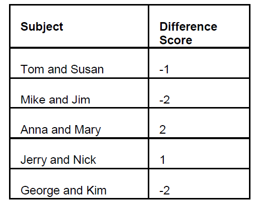
Mean for difference=0.4
The formula for the t-test for
dependent groups is

We read it as follows:
t for paired observations equals
mean of differences divided by the
standard deviation over the square
root of the n. (The standard
deviation divided by the square
root of the n is the standard error
of the mean, SEM, remember?)
You know all of the terms of the
t-formula. You also recognize that it
is the same old story, our old
friend, the z formula.
t=+0.49 df=4
Entering the t-table with df 10 we
find that the required t=2.132
Our obtained t 0.49 is smaller
than the required, therefore we do
not have significance. We say that
the difference we observed is not
significant (p>0.05).
Study the table below..
It adds to our effort toward integration
and understanding beyond a mechanistic
use of a plethora of formulas.
Study the table below..
It adds to our effort toward integration
and understanding beyond a mechanistic
use of a plethora of formulas.


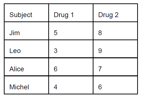
Example of ANOVA Repeated
Measures
Four patients with damage in the
hippocampus were treated with
two new drugs in order to see if
their memory improved.
Here is the layout as well as the
scores of the experiment. High
scores indicate improvement in
memory.
ANOVA SUMMARY TABLE
Repeated Measures
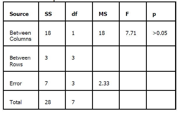
Entering the F table in Appendix
with df 1 and 3, we find an F of
10.12. This is the required F in
order to have significance. Our
obtained F (see ANOVA summary
table above) is 7.71. It is less than
the required F, therefore, we do
not have significance. We say:
There was no significant difference
between the means of the two
conditions (p>0.05).
P greater than point o five.
I see there are questions.
What is Between Columns? You ask.
It is the usual Between variance
that you know. The variance that
our treatments produce. The
variance of the means.
What is Between Rows? you ask.
If you look at the layout above,
you see that the rows are subjects,
one subject per row. The mean of
each subject is the mean of each
row. The variance of these means
are the variance between the
rows.
Why you did not calculate an F for
the Rows? you ask.
There is no reason that I can think
of, that would justify my wanting to
know whether there is a statistical
significant difference between
subjects. That would be an
absurd statement.
Once again you see that our
conceptual approach allowed us to
attack this design too, without the
need for new formulas. What is of
course more important is the fact
that we understand the logic of this
design too. We feel in command,
comfortable to handle any issue.
Story 17 — Example of a 2x3 factorial experiment
The layout of a 2x3 factorial ANOVA
In this example of a factorial design, we have a 2x3 (we read this as "a two by three") factorial. Two by three, meaning two factors: A and B. "two" meaning two levels for factor A. "three" meaning three levels for B. In another case of a 3x2 factorial design we have two factors, A and B, factor A three levels, factor B two levels.
FORMAT OF 2x3 FACTORIAL ANOVA SUMMARY TABLE
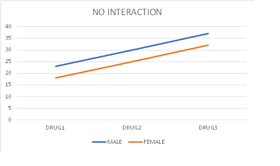
Interaction -factorial designs
Note the term "Interaction" in the ANOVA summary table of the factorial design What is interaction? The best way to grasp the concept of interaction is to graph it.
ANOVA 2x3 factorial practice example
An experimenter wanted to test the effect of two drugs on the emotionality of male and female teenagers. He randomly selected 15 male and 15 female teenagers and randomly assigned them to 6 groups: Group 1, Group 2, Group 3, Group 4, Group 5, Group 6. five subjects in each group as shown in the following table.
The data are presented on the table below. The scores are the values recorded on a device measuring galvanic skin response, a measure of emotionality. Higher values indicate stronger emotion.
.
2x3 FACTORIAL ANOVA SUMMARY TABLE
After we calculate the F, we go to the F table to find the required F value for A, B, and AxB (interaction). Because,( remember?) the F ratio is A over within, B over within,
AxB over within, we enter the F table with
df of A and df within , which is 1 and 24.
also B and df within, which is 2 and 24
and lastly AxB within., which is 2 and 24. We first choose the F table at 0.05 level of significance.
Factor A: The F at df 1 and 24 is 4.25. In the summary table we see that the F for factor A (rows) is 62.31. This is greater than 4.25, so we conclude that here we have significance at the 0.05 level of significance; we say p<0.05, p less than 0.05. It has been accepted among scientists that at the 0.05 level we are allowed to say that we have significance, that the finding of our experiment is reliable.
Next we look at factor B. We enter the F table with df 2 and 24 and find F=3.50. This is less than the F of our summary table 502.19, therefore we conclude that we have significance at the 0.05 level. We formally express this as follows: p<0.05.
Next we look at AxB. We enter the F table with df 2 and 24 and find F=3.50.. This is greater than the F at the summary table value of 1.75 so we conclude that here we do not have significance. We formally express this as follows: p>0.05.
Step by step calculation of 2x3 ANOVA factorial
The goal of our calculations in ANOVA is to compute the F ratio, The F ratio is MS between over MS within. Mean Square is the mean of the squared deviations (differences).
of each score from the mean. These are very simple calculations involving high school mathematics. Simple as they are, they are very important concepts in data analysis and beyond, that is science in general. You will never need to perform these calculations. There are many free Statistics calculators online. However, for the purpose of developing the concepts of ANOVA here are the steps:
1. Calculate the mean of each group.
2. Subtract each score from the mean.
3. Square each difference
4. Add these squared differences. font red This is the Sum of Squares, the SS on the ANOVA summary table.)
5. calculate the degrees of freedom df (number of scores that went into the calculation of the mean minus 1)
6 Divide the SS by the df. Voila! this the MS.
7. The last step is to calculate the F. Divide MS by the MS of the error term (which is the MS within but may be something else depending on which ANOVA design you have. )
The F ratio, as all ratios, compares two things. For example the ratio 8/4 compares 8 to 4 and finds that 8 is two times greater than 4.
Story 16B — Example 2 of a 2x2 factorial experiment
A pharmacology graduate student
working on his thesis wanted to
find whether a new chemical,
DOP-Y, which has been shown to
elevate dopamine levels in the
brain, may be beneficial to
depressive patients. He was also
interested to see if electroshock
has an effect on these patients
when combined with DOP-Y.
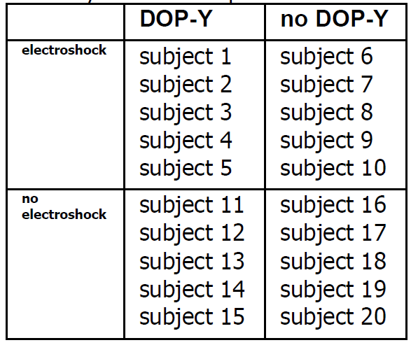
He randomly selected 20
depressive patients, and randomly
assigned them to 4 groups:
electroshock - DOP-Y,
electroshock-no DOP-Y
no-electroshock - DOP-Y,
no-electroshock-no DOP-Y
The layout of the pharmacology experiment

The data he recorded are given in
the next table.
The data of the pharmacology experiment

High numbers indicate improvement.
The data of the pharmacology experiment
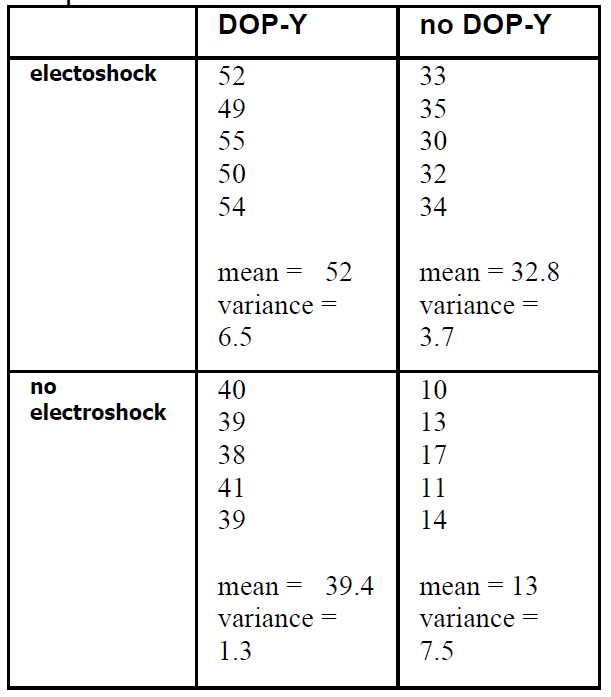
THE PHARMACOLOGY EXPERIMENT
ANOVA SUMMARY TABLE
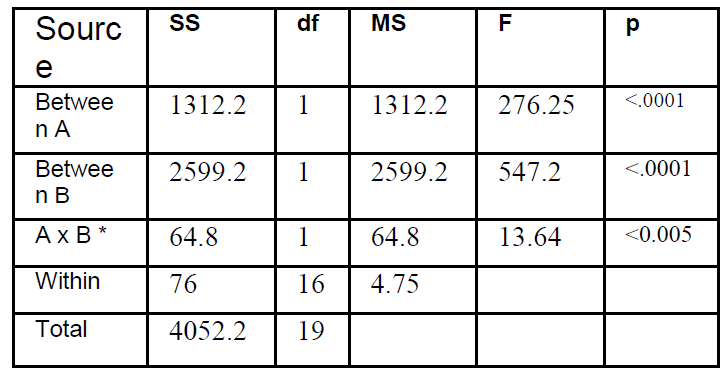
In this table we see that A, B, and
AxB are significant.
Significance in A means that
electroshock benefited the
depressive patients.
Significance in B means that drug
benefited the depressive patients.
Significance in AxB means that
there was an interaction between electroshock and drug.
Not clear, you say,
You are correct.
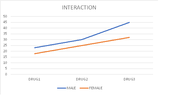
Let us look at the graph of the
interaction.
First, we observe that the two lines,
shock and no shock, are not
parallel. Every time we have an
interaction, the two lines are not
parallel.
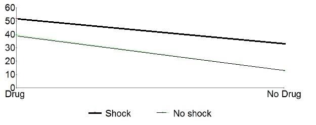
How about getting to understand
interaction at the gut level, not just
with words? you say.
Let’s do it. Look at the graph
above (previous page).
First, we will visualize the graph
without the effects of the drug. In
that graph the two lines would be
parallel.
Now visualize the effect of drug as
a force pushing the lines up.
Logically we would expect to see
both lines pushed up while
maintaining the distance between
them, i.e., the two lines may move
higher on the graph, but they
should remain parallel. However,
in the present experiment we saw
that the drug has pushed the no
electroshock line
disproportionately higher.
This is the concept of interaction.
Understanding the 2x2 factorial ANOVA summary table
A
Looking at the layout tables above, we see that factor A is gender. Factor B is drug. Our calculations gave a p value <0.05 meaning that factor A, gender, gave a significant difference. In other words, there is a difference in emotionality between male and female
B
Looking at the layout tables above, we see that factor B is Drug. Our calculations gave a p value <0.05, meaning that factor B, drug, gave a significant difference. In other words, there is a difference in emotionality between subjects that received drug 1 as compared to subjects that received drug 2.
AxB
This is the interaction term. Definition of the interaction. What is interaction in factorial designs? Interaction is present if one level of one factor has a disproportionate effect on one level of the other factor.
Story 16 — Examples of 2x2 factorial experiments ANOVA
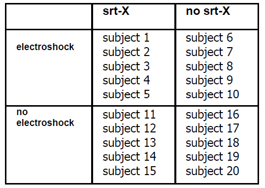
Example 1 of 2x2 factorial experiment ANOVA
A pharmacology graduate student
working on his thesis wanted to
find whether a new chemical,
srt-X, which has been shown to
block serotonin, may be beneficial
to schizophrenic patients. He was
also interested to see if
electroshock has an effect on
these patients when combined
with srt-X.
He randomly selected 20
schizophrenic patients, and
randomly assigned them to 4
groups:
electroshock - srt-X,
electroshock-no srt-X
no electroshock - srt-X,
no electroshock-no srt-X
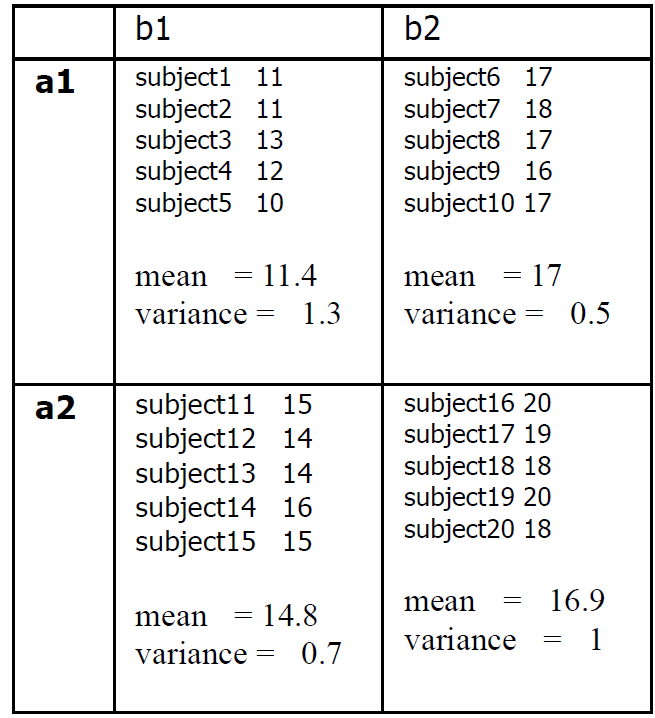
The layout of this experiment is:
The layout in abstract form is:
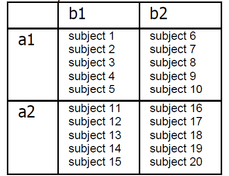
Variable A has two levels, a1 and
a2, and variable B has two levels,
b1 and b2.
The next table shows the data he
recorded in running the
experiment. The numbers
represent scores on a psychiatric
test measuring intensity of
schizophrenic behavior. The
higher the number the worse the
condition of the patient.
THE SEROTONIN BLOCKER
PLUS SHOCK EXPERIMENT
ANOVA SUMMARY TABLE OF
THE SEROTONIN BLOCKER
PLUS SHOCK EXPERIMENT
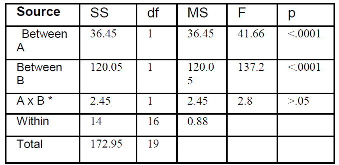
* Interaction
I will first discuss the table in terms
of the calculations we did.
First and most important, the
degrees of freedom.
If you tell me the degrees of
freedom in any ANOVA
experiment, but without the use of
formulas (I do also mean resorting
to memory for the recollection of
formulas - ban formulas!), I know
you know what you are talking
about. Calculation of the F is easy,
high school arithmetic.
If you
Why df for Between A is 1?
Because in order to calculate
variance Between we line up the
means, consider them scores, and
calculate the variance using the
one and only formula for variance
(all the other formulas for variance
that you may see around are
derived from this formula.
Statisticians get their kicks by
producing equivalent formulas, of
considerable complexity and
ornamental value!). Now you and I
know that in order to calculate
variance, we must first calculate
the mean. Every time we calculate
the mean, we lose 1 degree of
freedom. Because, in the present
example we have 2 scores (never
mind that they are means), we are
left with 1 df. That is 2-1=1.
I do not understand why you say
we have 2 means for A, you ask.
Good question. A has two levels
here, a1 and a2. That is shock and
no shock. You see, when we deal
with variable A, we ignore variable
B. In other words we reduce this
part of the analysis to a one-way,
single-factor ANOVA.
Why df for Between B is 1? you
say.
For the same reasons as in the
previous paragraph, B has two
levels, b1 and b2, drug and no
drug. There are two means
(scores). In order to calculate the
variance of these two scores, we
must first compute the mean. We
therefore lose 1 df. So the df for B
is 2-1=1.
Why df for AxB interaction is 1?
This is easy. Since df for A is 1, and
df for B is also 1, the df for AxB is
1x1=1.
Why is the df for within 16?
This is simple, too. We said variance
within is variance for the first
group plus variance for the second
group, plus variance for the third
groups and so on. We have four
groups here. In order to calculate
the variance of each group we
must first calculate a mean. The
consequence of this is that we
lose 1 df for every mean we
calculate. How many scores go
into the calculation of variance for
group 1? Five scores. Therefore
df for the first group is 5-1=4. We
calculate the variance of the
remaining 3 groups in a similar
way. Since we have 4 groups
here, the df for Within is 4x4=16.
he
Note: Checksum. The sum of df
for A, B, AxB, Within, equals df
Total
SS for A, B, AxB, and Within
equals SS Total.
Remember, we said that in ANOVA
we partition variance.
Discussion of the experiment
with the schizophrenic patients.
Look at the ANOVA Table again:
ANOVA SUMMARY TABLE OF
THE SEROTONIN BLOCKER
PLUS SHOCK EXPERIMENT
* Interaction
The p value (the probability that
the difference or effect we are
reporting may not be reliable or
significant) for A is less than 1 in
ten thousand (p<.0001|).
Variable A is electroshock in this
experiment. This means that the
two conditions, electroshock and
no electroshock (condition 1:
electroshock-drug, electroshock-no drug; condition 2: no-
electroshock-drug, no- electroshock-no drug) produced a result, a significant difference.
In other words those patients who received electroshock ended up different from those patients that did not receive electroshock.
The p value (the probability that the difference or effect we are reporting may not be reliable or significant) for B is less than 1 in ten thousand (p<.0001|).
Variable B is drug in this experiment. This means that the two conditions, drug and no drug (condition 1: drug-electroshock, drug-no electroshock, condition 2: no drug-electroshock, no drug-no electroshock) produced a result, a significant difference. In other words, those patients who received the drug were different from those patients that did not receive the drug.
The p value of AxB, the interaction
is p>.05, We read this as follows:
p greater than five per cent. This
means that if we were to say that
there was significant interaction
between electroshock and drug,
we would be running the chance
of reporting an effect that is not
reliable, not significant, meaning
that if we or someone else were to
do the same experiment again,
most likely would not find a
difference as we did
As we said earlier the concept of
interaction is a new one for us,
and we need to understand it our
way, at the gut level, as we are
used to.
We will now consider an experiment in which the interaction is significant.
Story 16 — Analysis of Variance Factorial Designs
Analysis of Variance
Factorial Designs
Two-Way ANOVA
The ANOVA that we discussed so
far is called 'One-way ANOVA' or
'Single-factor ANOVA'.
Now we will consider two-way
ANOVA or two-factor ANOVA.
The concepts we developed so far
also apply to two-way ANOVA.
What do you mean by one-way,
single-factor, two-way, or
two-factor? you say.
Drama
Beam storm
Rutgers College. May 9, 1999, 9:00 in the
morning. Two sections of Statistics 101 are in class: two adjacent classrooms, C120 and
C121. USS Spaceship Enterprise flew over the two classrooms and locked on the bio readings of the students. Then, classroom C120 was bombarded with a X-Z-LOBX beam for 10 milliseconds. The security cameras recorded an almost imperceptible tilt of the head to the left, while the professor of Statistics, without being aware, wrote the same complex formula for MS 5 times. Two nanoseconds after classroom C120 was bathed in the benevolent X-Z-LOBX beam, classroom C121 was bombarded by the same X-Z-LOBX beam for 100 milliseconds. All students raised the index finger of their right hand and stuck it in their left nostril. The professor started reciting the t-table but stopped short in a deluge of laughter from the students.
The duration of the students’ responses was
recorded by the spaceship and instantly
transmitted to Houston where a robot was
waiting to manually enter the data on the
layout of the experiment. The layout of the
experiment was made public, the data not.
Discussion of data was forbidden by a
unanimous decision of the Congress.
The layout of the USS Enterprise
experiment
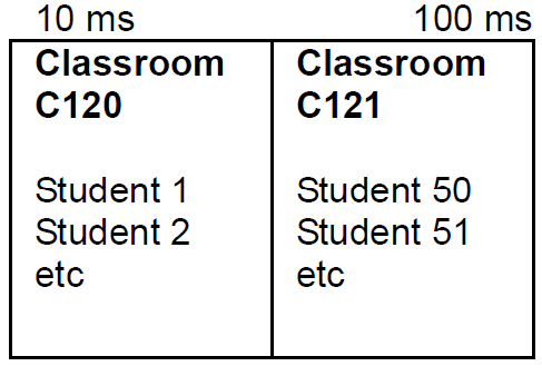
This experiment is a one-way
ANOVA design.
Why? Because each student was
bombarded with one beam.
We also say that this design is a
single-factor ANOVA.
Why?
Because each student was
bombarded with a single beam.
Another way of saying this is, that
each score in this experiment is
the result of one beam, one factor,
or one treatment. You may also
come across the term
one-way classification.
Now it will be easy for us to
understand two-way ANOVA.
An example of a two-way
ANOVA
A psychiatrist wanted to see
whether a combination of wine
and vitamin C may have an effect
on depression.
He randomly selected 10 male
patients, and also 10 female
patients, and randomly assigned
them in two groups: wine group, or
vitamin C group.
.
The layout of this experiment is
presented in the next table:
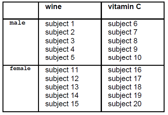
Look at subject 1. This subject is
influenced by two variables. Male
gender, and also wine. The score
of depression that he will give, will
be the result of these two factors.
For this reason, we call this type of
experiment a two-factor
experiment. The same, of course,
holds for all subjects. They are, in
a way, under crossfire. Two
factors hit them.
The layout above can also be
given in a more abstract form.
Variable A is gender, variable B is
nutrition. Each variable has two
levels, a1 a2 and b1 b2
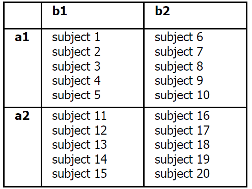
We say: We have two variables,
A and B. A is gender, B is nutrition.
Each of these two variables has
two levels. a1, a2, and b1, b2.
Because in this experiment we
use 2 variables with 2 levels each,
we call this experiment 2 x 2
factorial. We read this as follows:
two by two factorial.
The ANOVA summary table for
two-factor experiments is the
following:
ANOVA SUMMARY TABLE
Two-Way, 2x2 Factorial
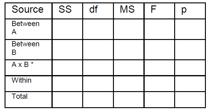
* Also called interaction
Things are getting complicated, I
hear you say.
I say: You already know everything
in this new ANOVA.
Our approach of understanding
the concepts and not memorizing
formulas has paid out.
Why do we have two Between
terms, A and B? you say.
Because here we have two
variables: gender, and nutrition,
i.e., A and B. We want to know if
gender (being male or female) has
an effect, and also if nutrition (wine
or vitamin C) has an effect.
Remember, the Between term is
the term that senses the effects of
our treatments.
The Within term we also know. It is
the variance of each group
separately. The sum of these
variances.
The Total term we also know. It is
simply the variance of all scores
without regard to what group they
came from.
The interaction term is a Between
term for cells taken diagonally:
mean for a1b1+a2b2 and mean
a1b2+a2b1. Look at the layout to
visualize this.
What is new here is the concept of
the interaction term. We need to
develop this concept, so we get a
gut feeling for it.
When you give two treatments to
subjects, one of the things you
want to see is whether the two
variables interact with each other.
To begin developing the concept
of interaction, let us consider a
simple experiment:
We give 5 mg of an anti-anxiety
drug, such as diazepam, and find
that this results in an increase in
the time patients sleep. This
increase is 2 hours.
Using different subjects, we find
that 200 ml of wine increase sleep
time by 1 hour.
Now if we give both 5 mg of
valium and 200 ml of wine, is it
sure that we will get 3 hours
increase in sleep time? Perhaps
yes, perhaps no. We know that
drugs may interact and produce
dramatic results, if given together.
You may have heard of cases in
which diazepam taken together
with alcohol caused coma, and
even death, because of
potentiation.
Students find the concept of
interaction difficult. For this reason
I will give an example later.
For the purposes of calculation of
this term in the ANOVA, there is no
problem. The df, as you would
expect, is the df of A x the df for B.
The SS you can calculate by
subtraction. SS total-(SS Between
A+SS Between B+SS within).
Alternatively, you can compute the
SS for AxB the same way you
calculated the between term, but
here calculate two means
diagonally, i.e.
mean for
a1b1+a2b2
and mean for
a2b1+a1b2.
Then we proceed with
the calculation of the variance of
these means.
The type of ANOVA design we are
discussing here is called factorial,
because in designing the
experiment we produce all
possible combinations.
In the above example we have:
Male - Wine, Male Vitamin C
Female - Wine, Female Vitamin C
Read this several times, it sounds
like a nursery rhyme. There is a
symmetry in it.
Visualizing the layout of
factorial designs
You will often come across
experiments that use these
designs, and if you go to graduate
school there is good chance you
will use them in your research.
We need to be able to visualize
the designs in order to understand
and evaluate them. A key
part of the task of a scientist is to
be able to critically evaluate the
research of others. Regrettably,
even reputable journals publish
research that is not sound.
We have considered so far a 2x2
design. How do we visualize this?
We see two characters (forget that
it is the number 2 here) separated
by the symbol x which stands for
times.
We have two things, two
variables, we therefore write down
A also B.
A B
Now we look again at 2x2 and this
time pay attention to what number
we have. Here we have 2.
We therefore write
A
a1 a2
Then we look at the number after
the x. It is also 2 (mind you it does
not have to always be 2, it can be,
4, 10 any number).
We therefore write
B
b1 b2
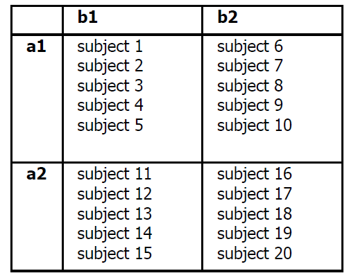
To sum up:
a1b1 a1b2
a2b1 a2b2
Read this several times, it sounds
like a nursery rhyme. There is a
symmetry in it.
This is how we visualize a 2x2
factorial:
a1b1 a1b2
a2b1 a2b2
Now let us consider this: 2x3 a1b2
a2a2b2
How do we visualize this? We
see two characters (forget that it is
the numbers 2 and 3 here)
separated by the symbol x which
stands for times. We have two
things, two variables, we therefore
write down A and also B.
A B
Now we look again at 2x3 and this
time pay attention to what
numbers we have. Before x we
have 2. We therefore write:
A
a1 a2
Then we look at the number after
the x. It is 3 (mind you, it does not
have to always be 3, it can be 4,
10, any number).
We therefore write:
B
b1 b2 b3
This is how we visualize a 2x3
factorial:
a1b1 a1b2 a1b3
a2b1 a2b2 a2b3
Now let us consider this: 2x3x5
How do we visualize this? We see
three characters (forget that it is
the numbers 2 and 3 and 5 here)
separated by the symbol x which
stands for times. We have three
things, three variables, we
therefore write down A, B,
also C.
A B C
Now we look again at 2x3x5 and
this time pay attention to what
numbers we have. Before x we
have 2.
We therefore write
A
a1 a2
Then we look at the number after
the x. It is 3 (mind you, it does not
have to always be 3, it can be, 4,
10, any number).
We therefore write
B
b1 b2 b3
Then we look at the third
number after the x. It is 5 (mind
you it does not have to always be
5, it can be, 6, 28, any number).
We therefore write
C
c1 c2 c3 c4 c5