

Goal. Test whether three teaching methods lead to different average exam scores.
Design & Experiment
Twenty-four students are randomly assigned to one of three methods (n = 8 per group):
- Group A: Active discussion
- Group B: Structured lecture
- Group C: Self-study
After a 2-week module, everyone takes the same 100-point exam.
Data
| Group A | Group B | Group C |
|---|---|---|
| 72 | 78 | 65 |
| 68 | 82 | 70 |
| 75 | 80 | 66 |
| 70 | 77 | 68 |
| 69 | 79 | 67 |
| 73 | 81 | 69 |
| 71 | 83 | 64 |
| 74 | 76 | 71 |
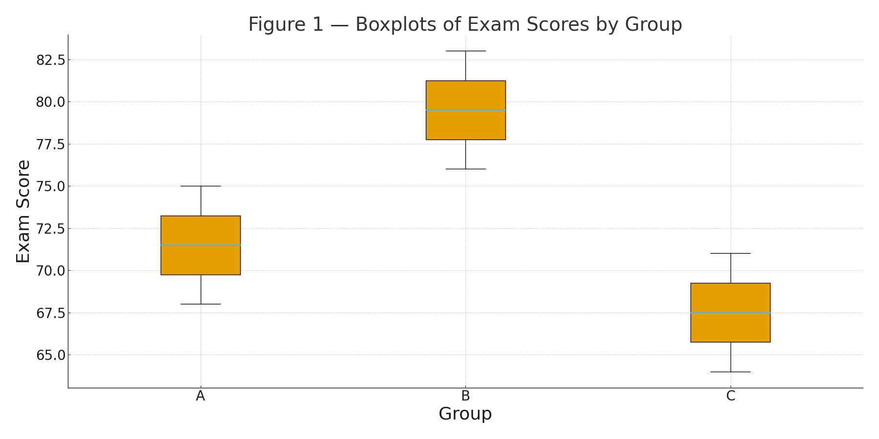
Figure 1: Boxplots of scores by group.
Group sizes: \(n_A=n_B=n_C=8\). Total \(N=24\).
Step 1 — Sums & Means
\(\displaystyle \begin{aligned} \text{Sums:}&\quad \sum A=572,\;\; \sum B=636,\;\; \sum C=540.\\[4pt] \text{Means:}&\quad \bar A=\tfrac{572}{8}=71.5,\;\; \bar B=\tfrac{636}{8}=79.5,\;\; \bar C=\tfrac{540}{8}=67.5.\\[4pt] \text{Grand mean:}&\quad \bar X=\tfrac{572+636+540}{24}=72.8333\ldots \end{aligned} \)
Step 2 — Within-Group Variability (sample variances)
For each group, compute \( s_g^2=\dfrac{\sum(x-\bar x_g)^2}{n_g-1} \).
- \(s_A^2 = 6.0\)
- \(s_B^2 = 6.0\)
- \(s_C^2 = 6.0\)
Corresponding sums of squares within each group: \(\displaystyle SS_A=\sum(x-\bar A)^2=42,\; SS_B=42,\; SS_C=42\Rightarrow SS_{\text{within}}=42+42+42=126.0. \)
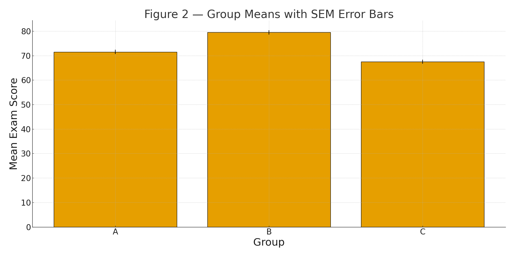
Figure 2: Group means with SEM error bars.
Step 3 — Between-Groups Variability
\(\displaystyle SS_{\text{between}}=\sum_{g} n_g(\bar x_g-\bar X)^2 =8(71.5-72.8333)^2+8(79.5-72.8333)^2+8(67.5-72.8333)^2 =597.3333\ldots \)
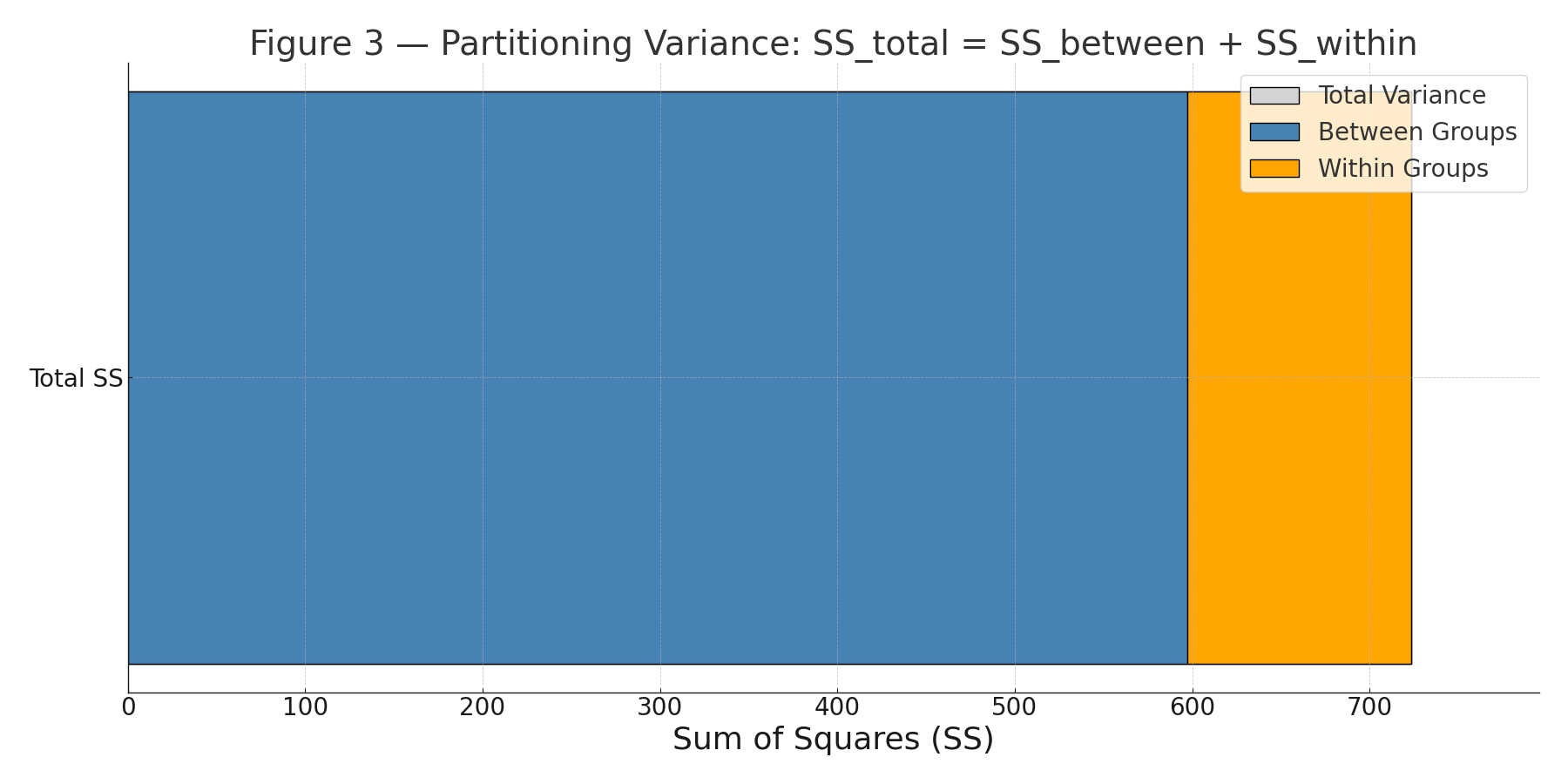
Total sum of squares: \(\displaystyle SS_{\text{total}}=\sum (x-\bar X)^2 = SS_{\text{between}}+SS_{\text{within}} =597.3333\ldots+126.0=723.3333\ldots \)
Figure 3: Partitioning variance (\(SS_{\text{total}}=SS_{\text{between}}+SS_{\text{within}}\)).
Degrees of Freedom & Mean Squares
\(\displaystyle df_{\text{between}}=k-1=3-1=2,\qquad df_{\text{within}}=N-k=24-3=21,\qquad df_{\text{total}}=N-1=23. \)
\(\displaystyle MS_{\text{between}}=\frac{SS_{\text{between}}}{df_{\text{between}}} =\frac{597.3333}{2}=298.6667,\qquad MS_{\text{within}}=\frac{SS_{\text{within}}}{df_{\text{within}}} =\frac{126.0}{21}=6.0. \)
Test Statistic & p-value
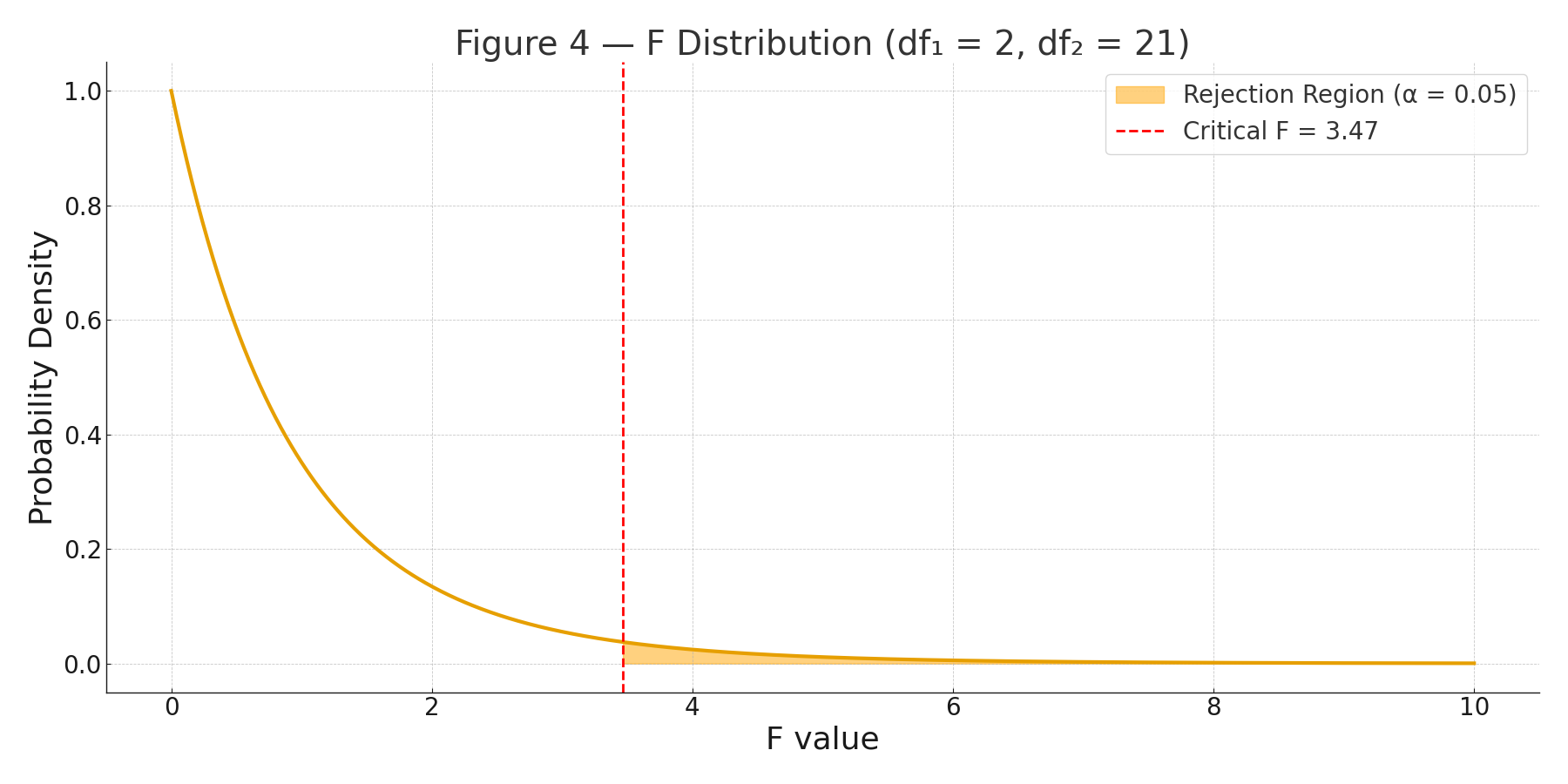
\(\displaystyle F=\frac{MS_{\text{between}}}{MS_{\text{within}}} =\frac{298.6667}{6.0}=49.7778. \)
With \(df_1=2\), \(df_2=21\), the (right-tail) p-value is \(p\approx 1.07\times10^{-8}\) (i.e., \(p<0.00000002\)).
Figure 4: F distribution curve with right-tail decision region.
ANOVA Summary Table
| Source | SS | df | MS | F | p |
|---|---|---|---|---|---|
| Between groups | 597.3333 | 2 | 298.6667 | 49.7778 | < 0.00000002 |
| Within (error) | 126.0000 | 21 | 6.0000 | — | — |
| Total | 723.3333 | 23 | — | — | — |
Conclusion
There is a statistically significant difference among the three methods’ mean scores (\(F(2,21)=49.78,\; p\ll .001\)). A post-hoc comparison (e.g., Tukey HSD) would identify which pairs differ.
Assumptions (checklist)
- Independent observations (via random assignment).
- Approximately normal scores within each group.
- Homogeneity of variance (here, each group variance \(\approx 6\)).
Practice self-test quiz
In the space below, please find practice problems and self-test quizzes. For full access, please signup free.