inferential-statistics

Simple regression predicts Y from one X.
But in real life, outcomes often depend on several variables — or may not be linear.

This chapter introduces multiple regression and logistic regression.

Multiple Regression

Formula:

$$\hat{Y} = a + b_1X_1 + b_2X_2 + \dots + b_kX_k$$

In words:
$$\text{Predicted Y} = \text{intercept} + (b_1 \times X_1) + (b_2 \times X_2) + \dots$$

Where:

• $$X_1, X_2, \dots X_k$$ = predictors
• $$b_1, b_2, \dots b_k$$ = slopes (weights for each predictor)

Example: Predicting college GPA from:

• High school GPA ($$X_1$$)
• Study hours ($$X_2$$)

Equation:
$$\hat{Y} = 1.0 + 0.5X_1 + 0.1X_2$$

Interpretation:

• For each 1-point increase in HS GPA, college GPA rises 0.5.
• For each extra study hour, GPA rises 0.1.

Coefficient of Determination

In multiple regression, $$R^2$$ tells us the proportion of variance explained by all predictors together.

Example: $$R^2 = 0.65$$ → predictors explain 65% of the outcome’s variability.

Logistic Regression

What if the outcome is yes/no (categorical)?
Example: Will a student pass or fail?

We use logistic regression.

Formula:

$$P(Y=1) = \frac{1}{1 + e^{-(a + bX)}}$$

In words:
$$\text{Probability of success} = \frac{1}{1 + e^{-(\text{intercept} + \text{slope} \times X)}}$$

Output: probability between 0 and 1.

Example: Predicting pass/fail from study hours.

• Equation: $$P = \frac{1}{1 + e^{-( -2 + 0.5X )}}$$
• If X = 6 hours: $$P = \frac{1}{1 + e^{-1}} = 0.73$$
• About 73% chance of passing.

Visuals

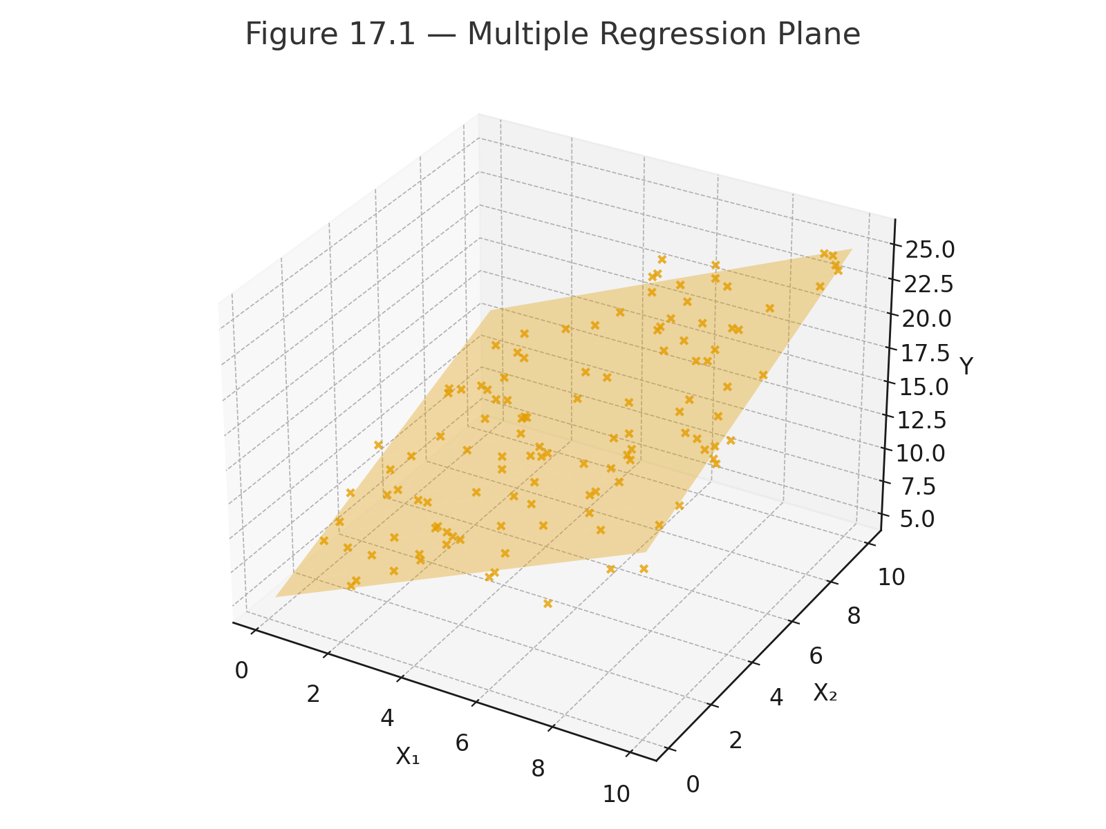
Figure 17.1 — Multiple regression plane: Y predicted from two predictors.

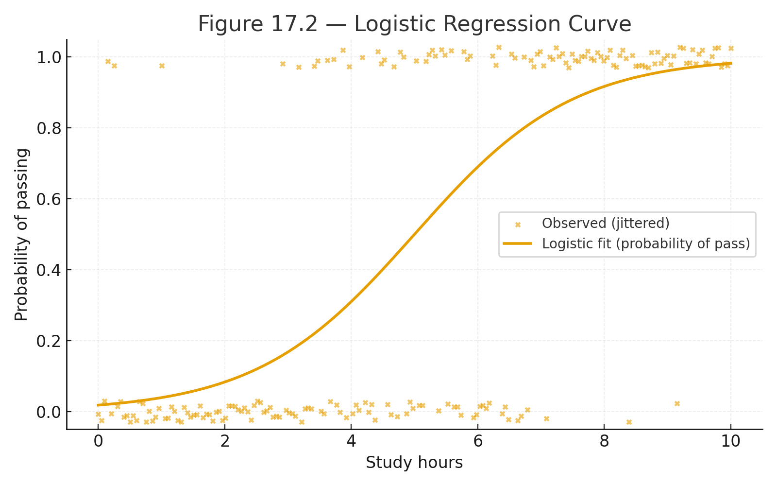
Figure 17.2 — Logistic regression curve: probability vs. study hours.

Why This Matters

• Multiple regression = prediction with many factors
• Logistic regression = prediction when the outcome is categorical
• $$R^2$$ = strength of prediction

These methods expand the power of regression beyond a straight line, preparing for modern predictive modeling.

Practice self-test quiz

In the space below, please find practice problems and self-test quizzes. For full access, please signup free.

Case 1 — Independent t-test (Two Groups)

Scenario: A teacher wants to compare math test scores between students taught with traditional lectures and those taught with interactive software.

Question: Are the two teaching methods different in average test score?

Design/Test: Independent-samples t-test.

Worked Example:

• Group A (Lecture): mean = 78, SD = 10, n = 20
• Group B (Software): mean = 85, SD = 12, n = 20

Formula:
$$t = \frac{\bar{X}_1 - \bar{X}_2}{\sqrt{\tfrac{s_1^2}{n_1} + \tfrac{s_2^2}{n_2}}}$$

In words:
$$t = \frac{\text{mean}_1 - \text{mean}_2}{\sqrt{\tfrac{\text{variance}_1}{n_1} + \tfrac{\text{variance}_2}{n_2}}}$$

Plugging in values:
$$t = \frac{78 - 85}{\sqrt{\tfrac{100}{20} + \tfrac{144}{20}}} = \frac{-7}{\sqrt{5 + 7.2}} = \frac{-7}{\sqrt{12.2}} = \frac{-7}{3.49} = -2.01$$

Degrees of freedom = 38.

Case 2 — Paired t-test (Before and After)

Scenario: Students take a memory test before and after a week of practice.

Question: Did memory scores improve after training?

Design/Test: Paired-samples t-test.

Worked Example:

Differences (After – Before): 2, 4, 3, 5, 6

• Mean difference:
  $$\bar{D} = \frac{2+4+3+5+6}{5} = 4$$
• Standard deviation of differences: $$s_D = 1.58$$

Formula:
$$t = \frac{\bar{D}}{s_D / \sqrt{n}}$$

Plugging in values:
$$t = \frac{4}{1.58/\sqrt{5}} = \frac{4}{0.71} = 5.63$$

Degrees of freedom = 4.

Case 3 — One-way ANOVA (Three Groups)

Scenario: A psychologist tests three methods of stress reduction: meditation, exercise, and music.

Question: Do the methods differ in average stress score?

Design/Test: One-way ANOVA.

Worked Example (summary):

• Group means: Meditation = 65, Exercise = 70, Music = 80
• $$SS_{\text{between}} = 300, , df_{\text{between}} = 2, , MS_{\text{between}} = 150$$
• $$SS_{\text{within}} = 200, , df_{\text{within}} = 12, , MS_{\text{within}} = 16.7$$

Formula:
$$F = \frac{MS_{\text{between}}}{MS_{\text{within}}}$$

Plugging in values:
$$F = \frac{150}{16.7} = 9.0$$

df = (2, 12).

Practice self-test quiz

In the space below, please find practice problems and self-test quizzes. For full access, please signup free.

The t-test compares two means. But what if we have three or more groups?
We could run multiple t-tests, but that inflates the chance of error.

The solution is the Analysis of Variance (ANOVA).
ANOVA partitions the variability into two parts: between groups and within groups.

Partitioning the Variance

Total variability = variability between groups + variability within groups.

• Between groups: differences due to the factor (treatment).
• Within groups: differences due to chance or individual variation.

Symbolic formula:
$$F = \frac{MS_{\text{between}}}{MS_{\text{within}}}$$

Formula in words:
$$F = \frac{\text{mean square between groups}}{\text{mean square within groups}}$$

Where:

• $$MS_{\text{between}} = \tfrac{SS_{\text{between}}}{df_{\text{between}}}$$
• $$MS_{\text{within}} = \tfrac{SS_{\text{within}}}{df_{\text{within}}}$$

Degrees of Freedom

• $$df_{\text{between}} = k - 1$$
• $$df_{\text{within}} = N - k$$
• $$df_{\text{total}} = N - 1$$

Where $$k$$ = number of groups, $$N$$ = total number of observations.

Example (One-way ANOVA)

Three groups of students use different study techniques:

• Group A: mean = 70
• Group B: mean = 75
• Group C: mean = 85

Suppose calculations give:

• $$SS_{\text{between}} = 300, , df_{\text{between}} = 2 \Rightarrow MS_{\text{between}} = 150$$
• $$SS_{\text{within}} = 200, , df_{\text{within}} = 12 \Rightarrow MS_{\text{within}} = 16.7$$

Then:

$$F = \frac{150}{16.7} = 9.0$$

This F value is compared to the F table at df = (2, 12).

Definition

• ANOVA: compares means across three or more groups.
• F ratio: signal-to-noise ratio (treatment effect vs. error).

Visual Placeholders

Figure L6.1 — Partitioning Variance. Total variability divided into Between vs. Within.

Figure L6.2 — One-way ANOVA Layout. Bar graph with three groups (A, B, C).

Figure L6.3 — ANOVA Summary Table. Source | SS | df | MS | F | p.

Why This Matters

ANOVA generalizes the t-test to multiple groups.
It is one of the most widely used tools in psychology, education, and medicine.
Understanding the F ratio is key: a large F means treatment differences are greater than chance variation. 

Practice self-test quiz

In the space below, please find practice problems and self-test quizzes. For full access, please signup free.

This lecture emphasizes conceptual understanding of the t-test, its logic, and how it fits into the broader structure of statistical reasoning.

The t-test is one of the most widely used statistical tools.
It compares two means and asks: Is the difference between them real, or could it be due to chance?

The t-test is closely related to the z-test.
When the population standard deviation is unknown and the sample size is small, we use t instead of z.

Types of t-Tests

• One-sample t-test: compares a sample mean to a known or hypothesized population mean.
• Independent-samples t-test: compares means from two separate groups.
• Paired-samples t-test: compares two scores from the same group (before vs. after).

Symbolic Formulas

One-sample t-test
$$t = \frac{\bar{X} - \mu_0}{s / \sqrt{n}}$$

Independent-samples t-test
$$t = \frac{\bar{X}_1 - \bar{X}_2}{\sqrt{\tfrac{s_1^2}{n_1} + \tfrac{s_2^2}{n_2}}}$$

Paired-samples t-test
$$t = \frac{\bar{D}}{s_D / \sqrt{n}}$$

Degrees of Freedom

• One-sample: $$df = n - 1$$
• Independent-samples: $$df = n_1 + n_2 - 2$$
• Paired-samples: $$df = n - 1$$

Example (Independent t-Test)

Two groups of students try different study methods:

• Group A: \(n = 10\), mean = 80, SD = 10
• Group B: \(n = 10\), mean = 90, SD = 10

$$t = \frac{80 - 90}{\sqrt{\tfrac{10^2}{10} + \tfrac{10^2}{10}}} = \frac{-10}{\sqrt{10 + 10}} = \frac{-10}{\sqrt{20}} = \frac{-10}{4.47} = -2.24$$

Degrees of freedom = 18.
Compare this t-value to the critical value in the t-table at \(df = 18\).

Example (Paired t-Test)

Students take a test before and after tutoring.
Differences (After − Before): 4, 6, 5, 3, 2.

Mean difference:
$$\bar{D} = \frac{4 + 6 + 5 + 3 + 2}{5} = 4$$

Standard deviation of differences:
$$s_D = 1.58$$

$$t = \frac{4}{1.58 / \sqrt{5}} = \frac{4}{0.71} = 5.63$$

Degrees of freedom = 4.
This large t-value indicates strong evidence of improvement.

Definition

• Independent t-test: compares two separate groups.
• Paired t-test: compares the same group measured twice.
• Degrees of freedom (df): number of independent pieces of information.

Visuals

Figure L5.1 — Independent t-Test. Bar graph of two groups (A and B) with means and SEM error bars.

Figure L5.2 — Paired t-Test. Line plot showing before vs. after scores for each student.

Figure L5.3 — t vs. z Distribution. Overlay of the normal (z) curve and t curves with df = 5 and 20.

Why This Matters

The t-test is the workhorse of statistics.
It forms the foundation for many other methods (ANOVA, regression, mixed models).
Understanding t means understanding how we compare signal (mean difference) to noise (variability).

Practice self-test quiz

In the space below, please find practice problems and self-test quizzes. For full access, please signup free.

The normal distribution is not just a shape — it is a powerful tool.
It allows us to describe data, calculate probabilities, and make decisions about means and differences.

Here are four major uses of the normal curve.

1. Describing Data

The normal curve summarizes how scores are distributed.

• Mean = center
• Standard deviation = spread

It provides a reference point: where most scores fall, and where extremes occur.

Figure L4.1 — Normal Curve with mean and ±1σ, ±2σ, ±3σ marked.

2. Probability of a Score

We can use the normal curve to calculate the probability of observing a score above or below a certain value.

Formula for standardization:
$$z = \frac{x - \mu}{\sigma}$$

Formula in words:
$$z = \frac{\text{score} - \text{mean}}{\text{standard deviation}}$$

The z-score tells us how many standard deviations a score is from the mean.
With the z-table, we can find the probability of that score.

Figure L4.2 — Normal curve with shaded area above z = 1.5.

3. Reliability of a Mean (SEM)

If we take many samples, the means vary. The Standard Error of the Mean (SEM) tells us how much.

Formula:
$$\mathrm{SEM} = \frac{s}{\sqrt{n}}$$

Formula in words:
$$\text{SEM} = \frac{\text{standard deviation}}{\sqrt{\text{number of scores}}}$$

Smaller SEM means the sample mean is a more reliable estimate of the population mean.

Figure L4.3 — Distribution of sample means, narrower than distribution of raw scores.

4. Reliability of a Difference

The normal distribution also underlies hypothesis testing — such as the t-test.
It allows us to compare two means and decide whether their difference is larger than expected by chance.

Figure L4.4 — Two overlapping normal curves with different means.

Why This Matters

The normal distribution is the foundation for:

• Calculating probabilities
• Estimating reliability of means
• Testing hypotheses about differences

Understanding these uses prepares us for the transition from descriptive to inferential statistics.

Practice self-test quiz

In the space below, please find practice problems and self-test quizzes. For full access, please signup free.

The mean tells us the “typical” score. But how tightly do scores cluster around the mean? Do they spread widely, or are they close together?

To answer, we measure variability. Two key measures are the variance and the standard deviation.

Variance

Variance is the average squared distance of scores from the mean.

Symbolic formula:
$$s^2 = \frac{\sum (X - \bar{X})^2}{n - 1}$$

Formula in words:
$$\text{Variance} = \frac{\text{sum of squared deviations from the mean}}{\text{number of scores} - 1}$$

Where:

• $$s^2$$ = variance
• $$X$$ = each score
• $$\bar{X}$$ = mean
• $$n$$ = number of scores

Standard Deviation

The standard deviation is the square root of the variance. It puts variability back into the same units as the data.

Symbolic formula:
$$s = \sqrt{\frac{\sum (X - \bar{X})^2}{n - 1}}$$

Formula in words:
$$\text{Standard deviation} = \sqrt{\frac{\text{sum of squared deviations from the mean}}{\text{number of scores} - 1}}$$

Example

Data: 6, 8, 10

• Mean = 8
• Deviations: –2, 0, 2
• Squared deviations: 4, 0, 4
• Sum = 8

Variance:
$$s^2 = \frac{8}{3-1} = 4$$

Standard deviation:
$$s = \sqrt{4} = 2$$

So, on average, scores are 2 units away from the mean.

Definition

• Variance: average squared distance from the mean.
• Standard Deviation: square root of variance; typical distance from the mean.

Visuals

Figure L3.1 — Variability Around the Mean. Dot plot of scores with the mean marked, vertical lines for deviations, and shaded boxes for squared deviations.

Why This Matters

Two sets of scores can have the same mean but very different spreads.
Variance and standard deviation give us the language to describe spread, and they are the building blocks for t-tests, ANOVA, and all inferential statistics.

Practice self-test quiz

In the space below, please find practice problems and self-test quizzes. For full access, please signup free.

The normal curve (bell curve) is one of the most important concepts in statistics.
It is elegant, symmetrical, and central to probability and inference.
It appears whenever many small, independent factors combine: height, exam scores, measurement errors.

Properties of the Normal Curve

1. Symmetrical around the mean
2. One peak (unimodal)
3. Mean = Median = Mode
4. Total area under the curve = 1 (100%)

Formula for the Normal Distribution

Symbolic formula:
$$f(x) = \frac{1}{\sigma \sqrt{2\pi}} e^{-\frac{(x - \mu)^2}{2\sigma^2}}$$

Formula in words:
$$\text{Probability density} = \frac{1}{\text{standard deviation} \times \sqrt{2\pi}} \times e^{-\frac{(\text{score} - \text{mean})^2}{2 \times (\text{standard deviation})^2}}$$

Where:

• $$\mu$$ = mean
• $$\sigma$$ = standard deviation
• $$x$$ = a score

Standardization (z-scores)

Symbolic formula:
$$z = \frac{x - \mu}{\sigma}$$

Formula in words:
$$z = \frac{\text{score} - \text{mean}}{\text{standard deviation}}$$

A z-score tells us how many standard deviations a score is above or below the mean.

Key Percentages

Under the normal curve:

• About 68% of scores are within 1 standard deviation of the mean
• About 95% are within 2 standard deviations
• About 99.7% are within 3 standard deviations

This is called the 68–95–99.7 rule.

Drama Box — “The Goddess Normal Curve”

Imagine a temple where a perfect curve stands tall — balanced and symmetrical.

• At the center is the mean, the balance point.
• Half of the people (data) stand on each side.
• As you move further away, fewer remain.
• The Goddess teaches fairness: most scores are near the center, extreme scores are rare.

This image helps students remember the normal curve not as a dry formula, but as a principle of balance and probability.

Visuals

Figure L2.1 — The Normal Curve. Bell-shaped curve centered at the mean (μ).

Figure L2.2 — The 68–95–99.7 Rule. Normal curve with shaded regions ±1σ, ±2σ, ±3σ.

Figure L2.3 — z-score Example. Normal curve with shaded area to the left of z = 1.0, labeled 0.8413.

Why This Matters

The normal curve is the foundation of inferential statistics.

• It allows us to calculate probabilities.
• It underlies t-tests, ANOVAs, and confidence intervals.
• It lets us compare scores across different tests and scales.

Practice self-test quiz

In the space below, please find practice problems and self-test quizzes. For full access, please signup free.