Story 9 — Normal distribution, Use number 1 To describe, to organize data

Michelangelo, Sistine Chapel

Point of contact.

God’s hand makes contact with the hand of

Man. Genesis. Magic moment. A whole

world begins here. The divine, the

immaterial, the perfect makes contact with

the earthly, imperfect, and imparts to it

some of the harmony of the spiritual, perfect

world.

Drama

Where does Basita fall?

Susan, our psychology professor,

decided to take a personal interest in the

learning of her students, and called

those scoring very low to her office.

Among those she called was Basita.

The bottom line of this is that you should

quit college immediately. You are the

bottom of the bottommost. You will

never be able to compete with other

college students. Find a job in a diner, in

a farm, anywhere, but do not waste your

time at college, she said to Basita.

The next day, Basita and her mother,

Mrs. Thinlips, an accountant by

profession, marched into Susan’s office.

I have already talked to your chairperson

about this. I demand that you explain to

me the basis of your criticism and absurd

advice to my daughter. You traumatized

her, in effect telling her that she is an

idiot. You will hear from my lawyer. For

now I want an explanation.

My daughter scored 45. The mean was

60. Forty-five is close to the mean, only

15 points below. Forty-five means that

Basita knows almost half of what you

expect her to know. Your telling my

daughter to quit college is most

unwarranted. I demand an explanation!

Mrs. Thinlips said, banging her fist on the

Susan’s desk.

Help, Susan said to herself, Goddess

Normal Curve, help. She brings out a

sizable cardboard model of the goddess

and bows.

Mrs., Thinlips, she said. The mean of the

scores in Basita’s class was indeed 60,

and the standard deviation was 5. Here

is the computer analysis.

Now we place 60 on the mean (0

standard deviation), that is in the middle

of the curve.

Flash, thunder, tempest winds,

Michelangelo hovers over the cardboard

model! Angels and ministers of heaven

and hell! Point of contact of the spiritual

with the material! A new science is born.

Statistics. All else is humble things after

the cosmogony of this moment of

Genesis. All subsequent statistical tests

bow to this archetypal creation.

We place 60 on the mean, that is in the

middle of the curve, Susan continues. Now

we move down to standard deviation -1,

to the first vertical line on the left of the

midline. This means that at this point we

have score 55. Now we move down one

more standard deviation, standard

deviation -2. Here we have score 50.

Finally, we move down one more standard

deviation, standard deviation -3. Here we

have score 45. This is Basita’s score. The

percentage of scores above this point is

99.865%. The lower-tail probability is about

0.135%, or roughly 1.35 out of 1000

students in expectation. This is not a fixed

maximum; observed counts vary from sample to

sample. Basita is still near the extreme lower tail. Imagine a line of 1000 students, a

small town, and your daughter standing at

the very end! Susan said, with a malicious

smile on her face.

Mrs. Thinlips or Basita have not been seen

on the campus ever since.

Back to our task to understand the

normal distribution, to understand

it our way, a gut-level

understanding.

In doing science we have two

domains, two worlds. The

empirical domain, the mud and

flesh domain, and the formal

domain, the domain of

abstractions, ideas, logic and

mathematics. The empirical

domain is our sense world, and

the data we get by running

experiments in it.

The formal domain is the world of

thought and mathematics.

Sciences progress by

superimposing perfect models of

mathematics on the imperfect,

variable, messy world of matter.

When we do that, we immediately

see things that we could not see

by looking only at the data we

have collected from observations

in the material world.

Newton succeeded in creating a

revolution in Physics by first

creating a calculus, which he

superimposed on nature. Galileo

Galilei, the man who started

science as we know it today, said

that the language of nature is

mathematics.

A most important note in Basita’s

story:

What if Basita’s score was not 45

but it was 43? How would we find

where it falls on the normal curve?

There is a formula called the z

formula. Here it is:

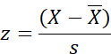
Let’s try it.

Score 43 minus the mean, which

is 60, equals -17. Now if we divide

-17 by the standard deviation

which is 5 here, we get a z of -3.4.

That makes sense. Basita’s score

of 45 fell exactly on standard

deviation -3, as we saw. A score of

43 will be even more to the left of

the curve.

I do not want to close this talk. I

want to play some triumphant

march, Beethoven’s Eroica

perhaps. Look at this formula. Play

with it, do things with it. Digest

what we do with it. Let’s dramatize

this.

Drama

An archetypal ceremony

I pick a score, and wave it in the

air. Then I wear my glasses and

stick my nose on the normal

curve, running up and down the

line with standard deviations on

it, I mumble:

Where does this score fall? Where

does this score fall?

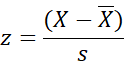
I then use the z formula and find

where exactly my score falls.

This is an archetypal ceremony.

Remember it. We will act it out

again in the future.

Story 8 — The uses of the normal distribution

You ask:

Why learn all these things about

the normal curve? What is the use

of all of this?

The use of all of this is necessary,

I say.

The normal curve (the standard normal curve) is a mathematical, perfect curve,

With magic qualities and powers.

Understanding the normal curve is

necessary, if we wish to

understand statistics from simple

t-tests to complex Analysis of

Variance (ANOVA).

The normal curve is used in four

instances:

1. To describe, to organize data.

2. To make statements regarding

probabilities as to the occurrence

of a particular score, as in games

of chance.

3. To make statements regarding

the reliability of a single mean

4. To make statements regarding

the reliability of the difference

between two means.

Understanding the concepts in

number 4 above is the basis for

understanding the concepts of all

statistical tests. Also, as we said

before, there is a continuity in the

process of our understanding of

statistics.

It is like a fairy tale. You must

know the full story, starting from

the beginning and step by step

reach the end, in order to make

sense. So keep alert!

Story 7 — Variance and standard deviation

Variance and standard deviation - intuitive level

Variance and standard deviation - formal level

Drama

Mathematical sweat

Susan Bolles is a new professor of

Psychology at Goatshead College.

Her chairman, sorry, chairperson, Dr.

Alexa Terrorvski, assigned her the

introductory psychology class of

1000 students. The first midterm

exam has just taken place. There

were 100 questions, 1 point each.

The exam papers were

computer-graded, all 1000 of them.

Dr. Terrorvski wants to know how

the class did, so she asks Susan.

Susan says that the mean (the

average) was 60.

Dr. Terrorvski wants to know more,

how many people scored close to

100, and how many people scored

close to zero. Susan walks up to the

pile of exam sheets and starts

reading the scores: 48, 30, 70, 99,

53 …… Papers are spread out from

the middle point, the average.

Realizing that this would take a good part

of the day, Dr. Terrorvski shouts out:

There must be a better way!

I will tell you what. Take this pile out to the

stadium, put it down in the middle of the

stadium. Mark this point 60 (your average

score). Take a step and mark this point 61.

Another step, mark this 62, all the way to

100. Return to mark 60 and take a step in

the opposite direction. Mark this point

59.Take another step, and mark this 58,

repeat all the way to mark 0. Now return to

your pile of exam sheets and pick up an

exam sheet. Read the score and walk to the

point it corresponds to on the markings you

made. I will return in an hour to see how

the exam went.

When Dr. Terrorvski returns she finds

Susan drenched in sweat and panting

vigorously. There is a long line of white

sheets of paper on both sides of the

point that marks 60, the average.

Susan picks up another exam sheet

which had the score of 3 and begins

walking. 59. 58. 57….

Enough! Terrorvski shouts. This is a

mess. Look at how many papers are

spread out away from the mean,

students have scored low scores, all

the way down to zero. So many

scores, so many students are very far

from 60, the mean. There is a big

distance of many scores from the

mean. You need to be more effective

in teaching your students, even the

weak ones, Dr. Terrorvski said, and

marched out of the stadium.

Susan went to her office and tried

to get a better picture of the

situation. Rather than walking

away from the point of the mean,

she calculated the distance of

each score from the mean. Score

40. Deviation from the mean: -20.

Score 65. Deviation from the mean:

+5. And so on. At the end she

added the absolute values of these distances and

she found the total absolute distance.

That was the distance she had to

walk in the stadium!

In the second midterm, the mean

was again 60. This time she did

not go out in the stadium. She

simply found out the distance of

each score from the mean. She

added the absolute values of these distances

and was pleased to see that the

total absolute distance was very small.

Surely, Dr. Terrorvski would not

yell at her this time. Students

scored close to the mean, there

were very few low scores. The

scores this time were not spread

out all over the place away from

the mean.

The symbol for variance is s².

The formula for variance is

\[ s^2=\frac{\sum (X-\bar{X})^2}{n-1} \]

We read this as follows:

Variance equals the sum of

squared deviations of each score

from the mean, divided by how

many scores went into the

calculation.

Why squared? Why square the

deviation, you say.

The sum of deviations from the

mean always, in all cases, equals

0. That is why we square each

deviation to prevent this. You

should know that in all sciences,

for the purpose of meaningful

analysis, we may transform our

data by squaring them, or

expressing them as logarithms,

and so on. This does not change

the relation of scores amongst

themselves.

Why divide by n-1 for a sample?

You understand that if in one case

we have large scores, and in

another small scores, the sum of

the deviations from the mean will

be large in the first instance, and

small in the second instance. If we

want to compare the spread of the

scores in the two instances, we

have to average each of these

sums of deviations. I hope you

understand this.

For example, in order to compare

the income of New Yorkers to

that of Chicagoans, we must

average the total income of New

Yorkers and Chicagoans.

The numerator of this formula

\[ \sum (X-\bar{X})^2 \]

is the sum of the difference of

each score squared, or raised to

the second power. More formally,

we say the numerator of the
variance formula is the sum of

squared deviations of each score from the

mean, squared. In statistical jargon

we say:

Sum of squares, or SS.

The numerator of the variance

formula is the

Sum of Squares,

or SS

For a sample, the denominator is n-1; for

an entire population, the denominator is N.

This converts the sum of squared deviations

into the appropriate sample or population

variance.

So, the variance formula is the

average of the sum of squared

deviations, or, in statistical jargon,

the mean squares or MS, for

short.

Variance is also called

mean squares

What is standard deviation? you say.

To calculate the standard deviation

we take the square root of

variance. Simple.

You do not need to know how to

calculate the square root of a

number. Not in the age of

computers. Anyone can learn to

do simple arithmetic. The

challenge is to understand

concepts of statistical and

mathematical operations.

The formula for standard deviation

is:

\[ s=\sqrt{s^2} \]

Do not worry about the -1 in the

denominator. The n changes

depending on whether we deal

with samples or an entire

population. Remember our goal

here is to understand the concepts

of statistics and want to avoid

getting stuck in compulsive

swamps.

We use n-1 when we work with samples.

We N without -1 when we refer to population.

Now that we have removed the

mystery of standard deviation of

the normal distribution, we return

to it.

Remember this is not just a curve,

it is Goddess Normal Curve. Glory

to NC in the highest!

Appendix 11: The F-Table (Critical Values at α = 0.05)

This table gives critical F-values for the F-distribution at the 5% significance level (one-tailed), used in ANOVA to test if group means differ significantly.

How to Use the F-Table

Left column: Degrees of freedom for the denominator (df₂ = df_within or error term).
Top row: Degrees of freedom for the numerator (df₁ = df_between or treatment term).
Find intersection value → that's the critical F.
If your calculated F > critical value → reject null hypothesis (significant difference at p < 0.05).

F Critical Values Table (α = 0.05)

**F Critical Values (α = 0.05)**
df₂ \ df₁	1	2	3	4	5	6	7	8	9	10
1	161.45	199.50	215.71	224.58	230.16	233.99	236.77	238.88	240.54	241.88
2	18.51	19.00	19.16	19.25	19.30	19.33	19.35	19.37	19.38	19.40
3	10.13	9.55	9.28	9.12	9.01	8.94	8.89	8.85	8.81	8.79
4	7.71	6.94	6.59	6.39	6.26	6.16	6.09	6.04	6.00	5.96
5	6.61	5.79	5.41	5.19	5.05	4.95	4.88	4.82	4.77	4.74
6	5.99	5.14	4.76	4.53	4.39	4.28	4.21	4.15	4.10	4.06
7	5.59	4.74	4.35	4.12	3.97	3.87	3.79	3.73	3.68	3.64
8	5.32	4.46	4.07	3.84	3.69	3.58	3.50	3.44	3.39	3.35
9	5.12	4.26	3.86	3.63	3.48	3.37	3.29	3.23	3.18	3.14
10	4.96	4.10	3.71	3.48	3.33	3.22	3.14	3.07	3.02	2.98
11	4.84	3.98	3.59	3.36	3.20	3.09	3.01	2.95	2.90	2.85
12	4.75	3.89	3.49	3.26	3.11	2.99	2.91	2.85	2.80	2.75
13	4.67	3.81	3.41	3.18	3.03	2.92	2.83	2.77	2.71	2.67
14	4.60	3.74	3.34	3.11	2.96	2.85	2.76	2.70	2.65	2.60
15	4.54	3.68	3.29	3.06	2.90	2.79	2.71	2.64	2.59	2.54
16	4.49	3.63	3.24	3.01	2.85	2.74	2.66	2.59	2.54	2.49
17	4.45	3.59	3.20	2.96	2.81	2.70	2.61	2.55	2.49	2.45
18	4.41	3.55	3.16	2.93	2.77	2.66	2.58	2.51	2.46	2.41
19	4.38	3.52	3.13	2.90	2.74	2.63	2.54	2.48	2.42	2.38
20	4.35	3.49	3.10	2.87	2.71	2.60	2.51	2.45	2.39	2.35
21	4.32	3.47	3.07	2.84	2.68	2.57	2.49	2.42	2.37	2.32
22	4.30	3.44	3.05	2.82	2.66	2.55	2.46	2.40	2.34	2.30
23	4.28	3.42	3.03	2.80	2.64	2.53	2.44	2.37	2.32	2.27
24	4.26	3.40	3.01	2.78	2.62	2.51	2.42	2.36	2.30	2.25
25	4.24	3.39	2.99	2.76	2.60	2.49	2.40	2.34	2.28	2.24
26	4.23	3.37	2.98	2.74	2.59	2.47	2.39	2.32	2.27	2.22
27	4.21	3.35	2.96	2.73	2.57	2.46	2.37	2.31	2.25	2.20
28	4.20	3.34	2.95	2.71	2.56	2.45	2.36	2.29	2.24	2.19
29	4.18	3.33	2.93	2.70	2.55	2.43	2.35	2.28	2.22	2.18
30	4.17	3.32	2.92	2.69	2.53	2.42	2.33	2.27	2.21	2.16
40	4.08	3.23	2.84	2.61	2.45	2.34	2.26	2.20	2.15	2.11

Example: One-Way ANOVA

Experiment: 3 groups, 10 subjects each → df_between = 2, df_within = 27. Calculated F = 12.54.

From table: df₂ = 27, df₁ = 2 → critical F ≈ 3.35.

Since 12.54 > 3.35 → significant difference (p < 0.05). Reject null hypothesis: At least one group mean differs.

Tip: For more precision, different α levels (e.g., 0.01), or larger df, use statistical software (Excel: F.INV.RT, Google Sheets, R: qf()). See Appendix 5 for technology tips.

Appendix 10: The t-Table (Critical Values for Student's t Distribution)

This appendix provides critical t-values for hypothesis testing (e.g., one-sample or independent t-tests) at common significance levels. Use it to determine if your calculated t-statistic indicates a significant difference (reject null hypothesis when |t| > critical value).

How to Use the t-Table

Left column: Degrees of freedom (df) — usually n-1 for one-sample or n₁ + n₂ - 2 for two independent samples.
Top row: Significance level (p, one-tailed or two-tailed depending on test).
Find the intersection value = critical t.
If your |calculated t| > critical t → reject null hypothesis (significant at that p level).
For two-tailed tests, use p/2 values (e.g., for α=0.05 two-tailed, use 0.025 column).

Example 1 (from page content)

Two independent groups, 10 subjects each → df = 18.

Calculated t = 4.51.

For a one-tailed test at α = 0.05, df = 18 gives critical t = 1.734. For a two-tailed test at α = 0.05, use the 0.025 column, giving critical t = 2.101.

In either case, 4.51 exceeds the critical value, so the result is significant (p < 0.05). Reject null hypothesis: means differ.

Example 2

One-sample t-test, n = 25 → df = 24.

Calculated t = 2.15.

Look up df = 24, p = 0.05 → critical t = 1.711 (one-tailed) or use 0.025 column = 2.064 (two-tailed).

If one-tailed: 2.15 > 1.711 → significant. If two-tailed: 2.15 > 2.064 → significant.

t Critical Values Table

**Student's t Critical Values**
df	0.10	0.05	0.025	0.01	0.005	0.001
1	3.078	6.314	12.706	31.821	63.657	318.31
2	1.886	2.920	4.303	6.965	9.925	22.326
3	1.638	2.353	3.182	4.541	5.841	10.215
4	1.533	2.132	2.776	3.747	4.604	7.173
5	1.476	2.015	2.571	3.365	4.032	5.893
6	1.440	1.943	2.447	3.143	3.707	5.208
7	1.415	1.895	2.365	2.998	3.499	4.782
8	1.397	1.860	2.306	2.896	3.355	4.499
9	1.383	1.833	2.262	2.821	3.250	4.296
10	1.372	1.812	2.228	2.764	3.169	4.143
11	1.363	1.796	2.201	2.718	3.106	4.024
12	1.356	1.782	2.179	2.681	3.055	3.929
13	1.350	1.771	2.160	2.650	3.012	3.852
14	1.345	1.761	2.145	2.624	2.977	3.787
15	1.341	1.753	2.131	2.602	2.947	3.733
16	1.337	1.746	2.120	2.583	2.921	3.686
17	1.333	1.740	2.110	2.567	2.898	3.646
18	1.330	1.734	2.101	2.552	2.878	3.610
19	1.328	1.729	2.093	2.539	2.861	3.579
20	1.325	1.725	2.086	2.528	2.845	3.552
21	1.323	1.721	2.080	2.518	2.831	3.527
22	1.321	1.717	2.074	2.508	2.819	3.505
23	1.319	1.714	2.069	2.500	2.807	3.485
24	1.318	1.711	2.064	2.492	2.797	3.467
25	1.316	1.708	2.060	2.485	2.787	3.450
26	1.315	1.706	2.056	2.479	2.779	3.435
27	1.314	1.703	2.052	2.473	2.771	3.421
28	1.313	1.701	2.048	2.467	2.763	3.408
29	1.311	1.699	2.045	2.462	2.756	3.396
30	1.310	1.697	2.042	2.457	2.750	3.385
40	1.303	1.684	2.021	2.423	2.704	3.307
60	1.296	1.671	2.000	2.390	2.660	3.232
∞	1.282	1.645	1.960	2.326	2.576	3.090

Tip: For exact p-values or larger df, use software (Excel: T.INV.2T, Google Sheets, R: qt()). See Appendix 5 for technology tips.

Appendix 9 — The normal distribution table

Appendix — The Normal Curve Table (Z-Table)

The Z-table (Standard Normal Distribution table) gives the area under the curve from the mean (z = 0) to a given z-score; it is not a left-tail cumulative-probability table. It is used in high school statistics to find probabilities, confidence intervals, and critical values for normal distribution problems.

How to Use the Z-Table

Left column: The z-score integer and first decimal (e.g., 1.9).
Top row: The second decimal place (0.00 to 0.09).
Find intersection → area from mean to that z-score (proportion of the distribution).
For negative z-scores, use symmetry (area is the same as positive).
For probability beyond z (tail), subtract from 0.5 (or 1 for two-tailed).

Example 1 (from page content)

z = 1.90 → row 1.9, column 0.00 → 0.4713. For z = 1.96, use row 1.9, column 0.06 → 0.4750.

Thus 47.13% lies between the mean and z = 1.90, and 47.50% lies between the mean and z = 1.96.

Example 2

Find probability that a score is less than z = 1.28 (e.g., for 90th percentile).

Row 1.2, column 0.08 → 0.3997.

Area from mean to z = 1.28 is 0.3997 → total area below z = 0.5 + 0.3997 = 0.8997 (≈90%).

Standard Normal (Z) Table — Cumulative Probabilities

**Cumulative Probabilities from Mean to z (Standard Normal Distribution)**
z	0.00	0.01	0.02	0.03	0.04	0.05	0.06	0.07	0.08	0.09
0.0	0.0000	0.0040	0.0080	0.0120	0.0160	0.0199	0.0239	0.0279	0.0319	0.0359
0.1	0.0398	0.0438	0.0478	0.0517	0.0557	0.0596	0.0636	0.0675	0.0714	0.0753
0.2	0.0793	0.0832	0.0871	0.0910	0.0948	0.0987	0.1026	0.1064	0.1103	0.1141
0.3	0.1179	0.1217	0.1255	0.1293	0.1331	0.1368	0.1406	0.1443	0.1480	0.1517
0.4	0.1554	0.1591	0.1628	0.1664	0.1700	0.1736	0.1772	0.1808	0.1844	0.1879
0.5	0.1915	0.1950	0.1985	0.2019	0.2054	0.2088	0.2123	0.2157	0.2190	0.2224
0.6	0.2257	0.2291	0.2324	0.2357	0.2389	0.2422	0.2454	0.2486	0.2517	0.2549
0.7	0.2580	0.2611	0.2642	0.2673	0.2704	0.2734	0.2764	0.2794	0.2823	0.2852
0.8	0.2881	0.2910	0.2939	0.2967	0.2995	0.3023	0.3051	0.3078	0.3106	0.3133
0.9	0.3159	0.3186	0.3212	0.3238	0.3264	0.3289	0.3315	0.3340	0.3365	0.3389
1.0	0.3413	0.3438	0.3461	0.3485	0.3508	0.3531	0.3554	0.3577	0.3599	0.3621
1.1	0.3643	0.3665	0.3686	0.3708	0.3729	0.3749	0.3770	0.3790	0.3810	0.3830
1.2	0.3849	0.3869	0.3888	0.3907	0.3925	0.3944	0.3962	0.3980	0.3997	0.4015
1.3	0.4032	0.4049	0.4066	0.4082	0.4099	0.4115	0.4131	0.4147	0.4162	0.4177
1.4	0.4192	0.4207	0.4222	0.4236	0.4251	0.4265	0.4279	0.4292	0.4306	0.4319
1.5	0.4332	0.4345	0.4357	0.4370	0.4382	0.4394	0.4406	0.4418	0.4429	0.4441
1.6	0.4452	0.4463	0.4474	0.4484	0.4495	0.4505	0.4515	0.4525	0.4535	0.4545
1.7	0.4554	0.4564	0.4573	0.4582	0.4591	0.4599	0.4608	0.4616	0.4625	0.4633
1.8	0.4641	0.4649	0.4656	0.4664	0.4671	0.4678	0.4686	0.4693	0.4699	0.4706
1.9	0.4713	0.4719	0.4726	0.4732	0.4738	0.4744	0.4750	0.4756	0.4761	0.4767
2.0	0.4772	0.4778	0.4783	0.4788	0.4793	0.4798	0.4803	0.4808	0.4812	0.4817
2.1	0.4821	0.4826	0.4830	0.4834	0.4838	0.4842	0.4846	0.4850	0.4854	0.4857
2.2	0.4861	0.4864	0.4868	0.4871	0.4875	0.4878	0.4881	0.4884	0.4887	0.4890
2.3	0.4893	0.4896	0.4898	0.4901	0.4904	0.4906	0.4909	0.4911	0.4913	0.4916
2.4	0.4918	0.4920	0.4922	0.4925	0.4927	0.4929	0.4931	0.4932	0.4934	0.4936
2.5	0.4938	0.4940	0.4941	0.4943	0.4945	0.4946	0.4948	0.4949	0.4951	0.4952
2.6	0.4953	0.4955	0.4956	0.4957	0.4959	0.4960	0.4961	0.4962	0.4963	0.4964
2.7	0.4965	0.4966	0.4967	0.4968	0.4969	0.4970	0.4971	0.4972	0.4973	0.4974
2.8	0.4974	0.4975	0.4976	0.4977	0.4977	0.4978	0.4979	0.4979	0.4980	0.4981
2.9	0.4981	0.4982	0.4982	0.4983	0.4984	0.4984	0.4985	0.4985	0.4986	0.4986
3.0	0.4987	0.4987	0.4987	0.4988	0.4988	0.4989	0.4989	0.4989	0.4990	0.4990

Tip: For negative z-scores, the area is the same (symmetry). For tail probabilities, subtract from 0.5 (one-tailed) or 1 (two-tailed). Use software for exact values (Excel: NORM.S.DIST, Google Sheets, R: pnorm()). See Appendix 5 for technology tips.

About | High School Statistics (Pre-College)

About This Textbook

Statistics for High School Students: Pre-College is a free, broad-ranging, and interactive online textbook written by Dr. Michael Nikoletseas—a professor and researcher with numerous publications in neuroscience, philosophy of science, and mathematics. Using mainly elementary arithmetic, straightforward formulas, and plain English, this resource is designed to be highly accessible. Despite its simplicity, it covers both elementary and advanced statistics topics, as well as modern data science concepts.

Mission & Vision

Our mission is to deliver a statistics textbook that:

supports students across a wide range of disciplines (from social and behavioral sciences to engineering and mathematics) to acquire a deep understanding of statistical reasoning, not just procedural techniques;
presents key statistical concepts in a manner that bridges theory and practice, emphasizing interpretive insight (“what does this mean?”) alongside computational method;
adopts an open mindset toward pedagogy: the site is structured for readability, modular use (individual chapters may be used independently if desired), and easy updates as the field evolves;
integrates modern elements—resampling, simulation, machine learning prelude, robust inference—while preserving the classical foundations (distributions, hypothesis testing, ANOVA, regression) so students are well‐grounded for further work.

Who This is For

This textbook is ideal for:

high school students preparing for biology or social science majors.
students in a one- or two-semester introductory statistics sequence who want more than formula memorization;
non‐mathematics majors (e.g. philosophy of science) who need to understand how to interpret and apply statistical reasoning in their discipline;
mathematics or statistics majors seeking a readable, web‐enabled resource that complements more formal references;
educators who want a ready‐to-use, modular, up‐to‐date resource for their course, including figures, examples, and modern topics.

Author & Credentials

Dr Michael Nikoletseas is the author of this textbook and brings a unique interdisciplinary background: his published works span neuroscience, philosophy of science, and mathematics, and are held in leading academic libraries (Harvard, Oxford, Princeton). His ambition with this text is to raise the bar for clarity, coherence, and depth in undergraduate statistics education.

With this online text, he applies the same analytical rigor he uses in his philosophical and mathematical writing: clear definitions, structured exposition, precise notation, and an emphasis on the limits of inference and interpretation (a theme that resonates with his broader work in epistemology).

Structure of the Textbook

The book is arranged into chapters each designed to stand on its own while also fitting into an integrated whole. Typical chapters will proceed in this order:

Introduction & motivation
Essential theory and notation for mathematics and formulas)
Detailed examples and figures (copyable images for instructor use)
Worked problems, with step-by-step solutions and commentary
Live self-test quizzes
Ask questions in each chapter
Advanced topics, extensions, and links (for students preparing for further study)

Current chapters already include: descriptive statistics, probability, distributions, the normal distribution, hypothesis testing, t‐tests, one‐way and multi‐way ANOVA (including mixed designs and post-hoc comparisons), resampling and simulation, machine learning foundations, and big data computational statistics.

Contact & Feedback

Your feedback is valuable. Should you spot an error, have a suggestion for improvement or want to request supplementary material use Feedback on main menu. Use the contact form below each chapter to ask questions.

Acknowledgements

The creation of this textbook has drawn on countless influences—from classical mathematics and modern statistics pedagogy to insights from neuroscience, philosophy of science, and epistemology. Special thanks to readers and educators who engage with the text, write with questions, and propose improvements. Together we advance statistical literacy and interpretive clarity.

Thank you for visiting StatisticsTextbook.com. May this textbook serve you well in your statistical journey.

— Michael Nikoletseas

Students

For Students: How to Use statisticstextbook.com

A simple guide for starting, studying in order, and reviewing.

Audience: Pre-college and high school students

October 20, 2025

1. What This Site Is

statisticstextbook.com is a free, page-by-page statistics textbook. You can read it in order like a print book, or use it as a reference when you need help with a topic.

Most students do best by moving from the foundations (data, variability, probability) into core tests (t-tests and ANOVA), and then into modern topics (resampling, big data, and an introduction to machine learning).

2. How to Use This Textbook

Start with the first lesson.
- Lesson 1: What Is Statistics? Why Does It Matter?
Follow the Next / Previous links. Each lesson ends with navigation links so you can keep the correct order without guessing what comes next.
Keep a small “definitions” page in your notes. Write down the meaning of key terms (mean, variance, standard deviation, probability, distribution) as you encounter them.
For each test, practice three skills. (1) what the question is, (2) the computation, (3) the interpretation in words.
Use the review pages when you get stuck.
- Appendix 2 — Math Review for Statistics
- Lesson 4 — The Standard Normal Curve

3. Reading the Math

Formulas are displayed with MathJax so they stay clear on different screens. If a formula looks unfamiliar, read it slowly and connect each symbol to a meaning in words.

4. Why This Format Helps

Clear sequence: lessons build from basic ideas to core tests.
Readable math: formulas render cleanly across devices.
Study-friendly: minimal distractions and no sign-in required.
Open access: free to use for learning and review.

5. Summary

Use the textbook in order if you are learning statistics for the first time, and use it as a reference when you need a quick explanation or a worked example. If you study steadily and keep your own notes of definitions and interpretations, the material becomes much easier over time.

Mixed (Split-Plot) ANOVA

Goal. Test a between-subjects factor (Group: Drug vs. Placebo) and a within-subjects factor (Time: Weeks 1–3), plus their interaction, on exam scores.

Design & Experiment

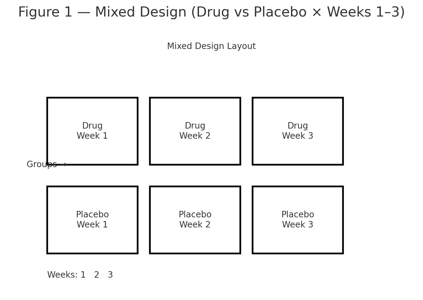
Between-subjects factor: Group = {Drug, Placebo}
Within-subjects factor: Time = {Week 1, Week 2, Week 3}
Balanced: 8 participants per group (\(s_g=8\)), 3 repeated measures per participant (\(k=3\)).

Participants are randomly assigned to Drug or Placebo. The same exam is given at Week 1, Week 2, and Week 3.

Figure 1: Mixed design layout (Drug vs Placebo × Weeks 1–3).

Data

Group: Drug (8 participants × 3 weeks)

Subject	W1	W2	W3	Row sum	Row mean
D1	70	74	78	222	74.00
D2	69	73	77	219	73.00
D3	71	75	79	225	75.00
D4	72	76	80	228	76.00
D5	68	72	76	216	72.00
D6	70	74	78	222	74.00
D7	73	77	81	231	77.00
D8	71	76	80	227	75.67
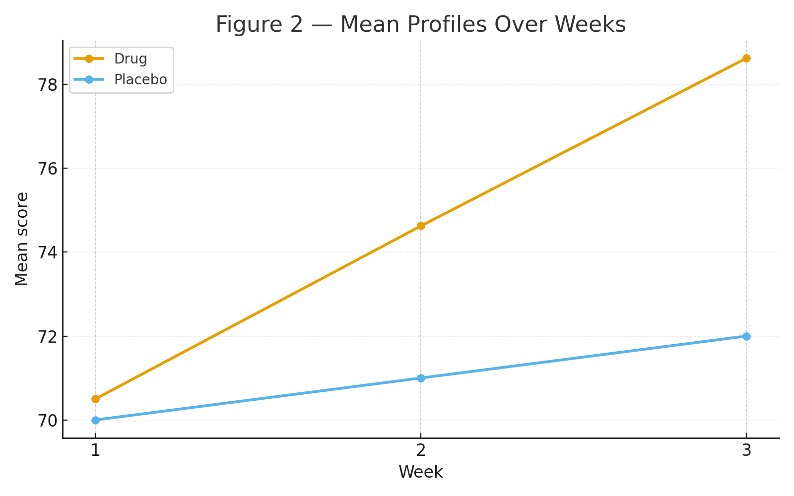
Column sums	564	597	629	Group sum = 1790	Group mean \( \bar X_{\text{Drug}} = 1790/24 = 74.5833 \)

Group: Placebo (8 participants × 3 weeks)

Subject	W1	W2	W3	Row sum	Row mean
P1	70	71	72	213	71.00
P2	69	70	71	210	70.00
P3	71	72	73	216	72.00
P4	72	73	74	219	73.00
P5	68	69	70	207	69.00
P6	70	71	72	213	71.00
P7	69	70	71	210	70.00
P8	71	72	73	216	72.00
Column sums	560	568	576	Group sum = 1704	Group mean \( \bar X_{\text{Plac}} = 1704/24 = 71.0000 \)

Totals. Grand sum = 1790 + 1704 = 3494, total observations \(N = 16\times3 = 48\), grand mean \( \bar X = 3494/48 = 72.7917\).

Figure 2: Mean profiles over weeks (Drug rises sharply; Placebo ~ flat).

Step 1 — Marginal Means

By Time (across both groups; 16 participants each week): \[ \bar X_{\text{W1}}=\tfrac{1124}{16}=70.2500,\qquad \bar X_{\text{W2}}=\tfrac{1165}{16}=72.8125,\qquad \bar X_{\text{W3}}=\tfrac{1205}{16}=75.3125, \] where column sums are \(1124, 1165, 1205\).

By Group (across all weeks): \[ \bar X_{\text{Drug}}=74.5833,\qquad \bar X_{\text{Placebo}}=71.0000. \]

Step 2 — Sums of Squares (SS)

Decompose total variability into Between-Subjects and Within-Subjects parts.

2A. Total

\[ SS_{\text{total}}=\sum (X_{igt}-\bar X)^2=\mathbf{527.9167}. \]

2B. Between-Subjects

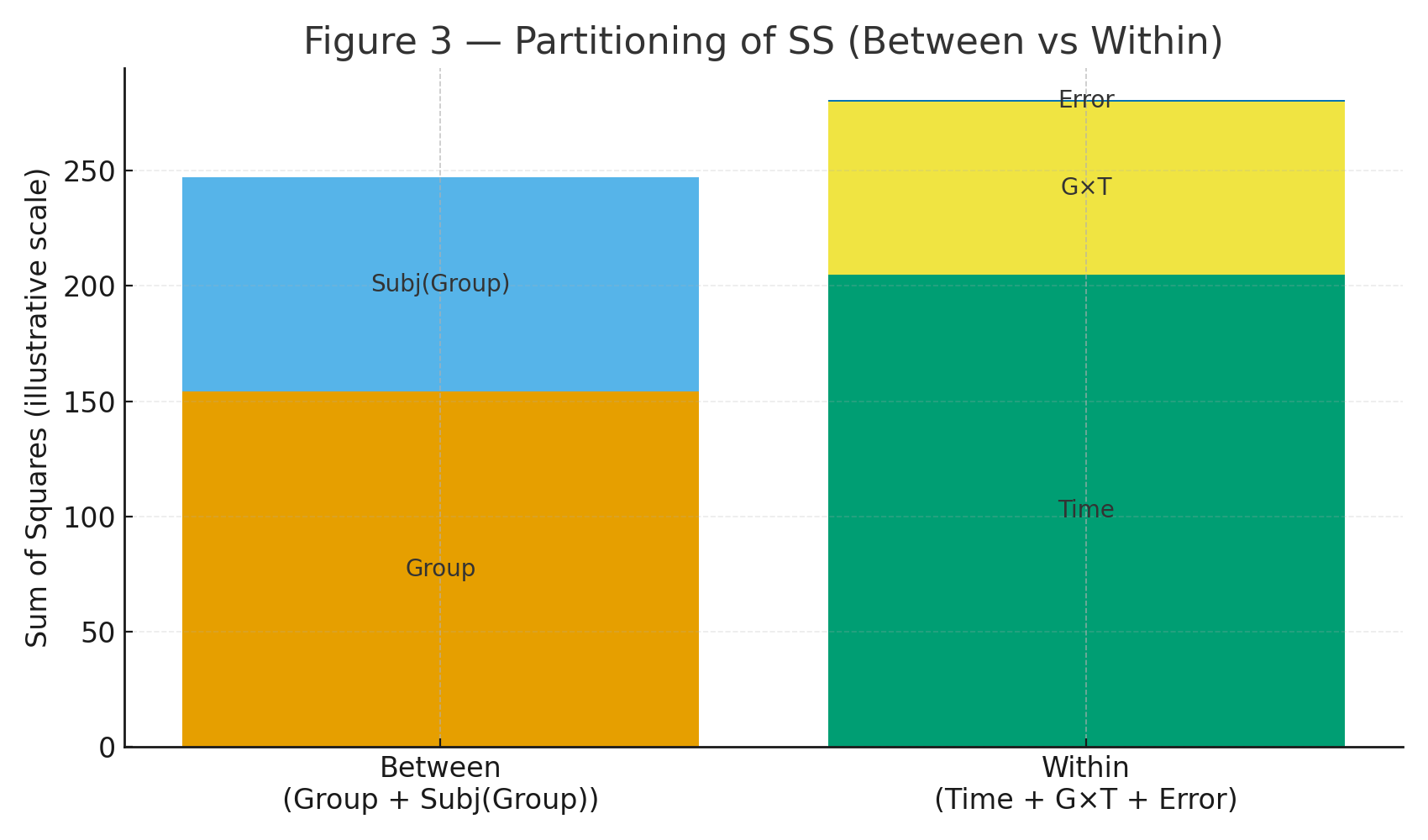
Let each subject’s mean be \(\bar X_{i\cdot}\). Then \[ SS_{\text{BS-total}}=k\sum_{i=1}^{16}(\bar X_{i\cdot}-\bar X)^2=\mathbf{247.2500}. \] Split into Group and Subjects-within-Group: \[ SS_{\text{Group}}=k\sum_{g} n_g(\bar X_{g\cdot\cdot}-\bar X)^2=\mathbf{154.0833}, \] \[ SS_{\text{Subj}(g)}=k\sum_{i\in g}(\bar X_{i\cdot}-\bar X_{g\cdot\cdot})^2=\mathbf{93.1667}. \]

2C. Within-Subjects

\(SS_{\text{WS-total}}=SS_{\text{total}}-SS_{\text{BS-total}}=\mathbf{280.6667}.\)

Decompose into Time, Group×Time, and residual Error: \[ SS_{\text{Time}}=s\sum_{t}(\bar X_{\cdot\cdot t}-\bar X)^2=\mathbf{205.0417}, \] \[ SS_{\text{Group}\times\text{Time}} =\sum_{g,t} n_g\Big(\bar X_{g\cdot t}-\bar X_{g\cdot\cdot}-\bar X_{\cdot\cdot t}+\bar X\Big)^2 =\mathbf{75.0417}, \] \[ SS_{\text{Error(WS)}}=SS_{\text{WS-total}}-SS_{\text{Time}}-SS_{\text{G}\times\text{T}} =\mathbf{0.5833}. \]

Figure 3: Partitioning diagram (Between: Group + Subj(Group); Within: Time + G×T + Error).

Step 3 — Degrees of Freedom (df) & Mean Squares (MS)

\[ \begin{aligned} &df_{\text{Group}}=g-1=1,\qquad df_{\text{Subj}(g)}=N_s-g=16-2=14,\\ &df_{\text{Time}}=k-1=2,\qquad df_{\text{G}\times\text{T}}=(g-1)(k-1)=2,\\ &df_{\text{Error(WS)}}=(N_s-g)(k-1)=(16-2)\times2=28,\\ &df_{\text{Total}}=Nk-1=48-1=47. \end{aligned} \]

\[ \begin{aligned} &MS_{\text{Group}}=\frac{SS_{\text{Group}}}{df_{\text{Group}}}= \frac{154.0833}{1}= \mathbf{154.0833},\qquad MS_{\text{Subj}(g)}=\frac{93.1667}{14}= \mathbf{6.6548},\\ &MS_{\text{Time}}=\frac{205.0417}{2}= \mathbf{102.5208},\qquad MS_{\text{G}\times\text{T}}=\frac{75.0417}{2}= \mathbf{37.5208},\\ &MS_{\text{Error(WS)}}=\frac{0.5833}{28}= \mathbf{0.02083}. \end{aligned} \]

Step 4 — F Tests & p-values

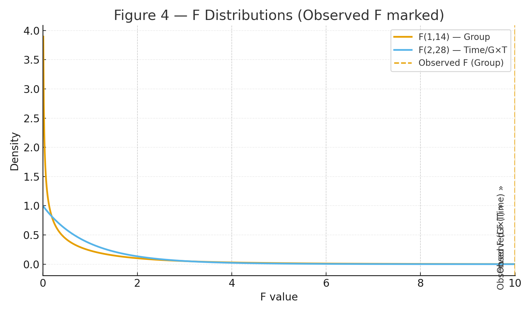
Between-subjects test: \[ F_{\text{Group}}=\frac{MS_{\text{Group}}}{MS_{\text{Subj}(g)}}=\frac{154.0833}{6.6548}= \mathbf{23.1538}, \quad df=(1,14),\quad p\approx \mathbf{0.00028}. \]

Within-subjects tests: \[ F_{\text{Time}}=\frac{MS_{\text{Time}}}{MS_{\text{Error(WS)}}} =\frac{102.5208}{0.02083}= \mathbf{4921.0},\quad df=(2,28),\quad p\ll 10^{-20}. \] \[ F_{\text{G}\times\text{T}}=\frac{MS_{\text{G}\times\text{T}}}{MS_{\text{Error(WS)}}} =\frac{37.5208}{0.02083}= \mathbf{1801.0},\quad df=(2,28),\quad p\ll 10^{-20}. \]

Figure 4: F distributions with observed statistics marked.

Mixed ANOVA Summary Table

Source	SS	df	MS	F	p
Between: Group	154.0833	1	154.0833	23.1538	0.00028
Between: Subjects within Group	93.1667	14	6.6548	—	—
Within: Time	205.0417	2	102.5208	4921.0	< 1e-20
Within: Group × Time	75.0417	2	37.5208	1801.0	< 1e-20
Within: Error (Subj×Time within Group)	0.5833	28	0.02083	—	—
Total	527.9167	47	—	—	—

Interpretation

Group: Drug > Placebo overall (significant between-subjects effect).
Time: Scores increase across weeks (strong within-subjects effect).
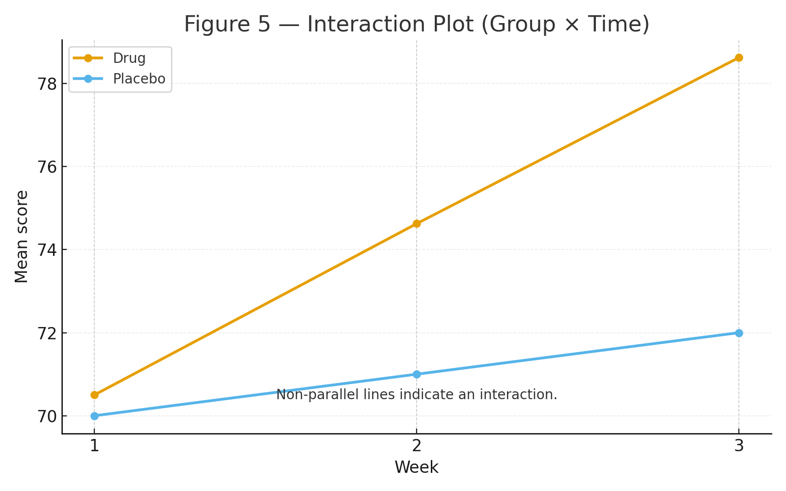
Group × Time: The Drug group improves sharply week-to-week while the Placebo group changes little (significant interaction).

Figure 5: Interaction plot showing non-parallel lines (Drug rising; Placebo flat).

Assumptions (checklist)

Independence between subjects; correct grouping.
Approximate normality within each Group×Time cell.
Homogeneity of variance across groups (between-subjects).
Sphericity for the within-subject factor Time (apply Greenhouse–Geisser/Huynh–Feldt corrections if violated).

Note: The residual within-subject error is intentionally small in this teaching dataset, so the Time and G×T F values are very large. Real data typically have larger residual variability.

Practice self-test quiz

In the space below, please find practice problems and self-test quizzes. For full access, please signup free.

Repeated-Measures ANOVA

Goal. Test whether performance changes across four conditions measured on the same participants.

Design & Experiment

Within-subjects factor: Condition with 4 levels (C1, C2, C3, C4).
s = 8 participants measured in k = 4 conditions ⇒ total observations \(N = s \times k = 32\).
Example context: the same students take four weekly quizzes after different study activities.

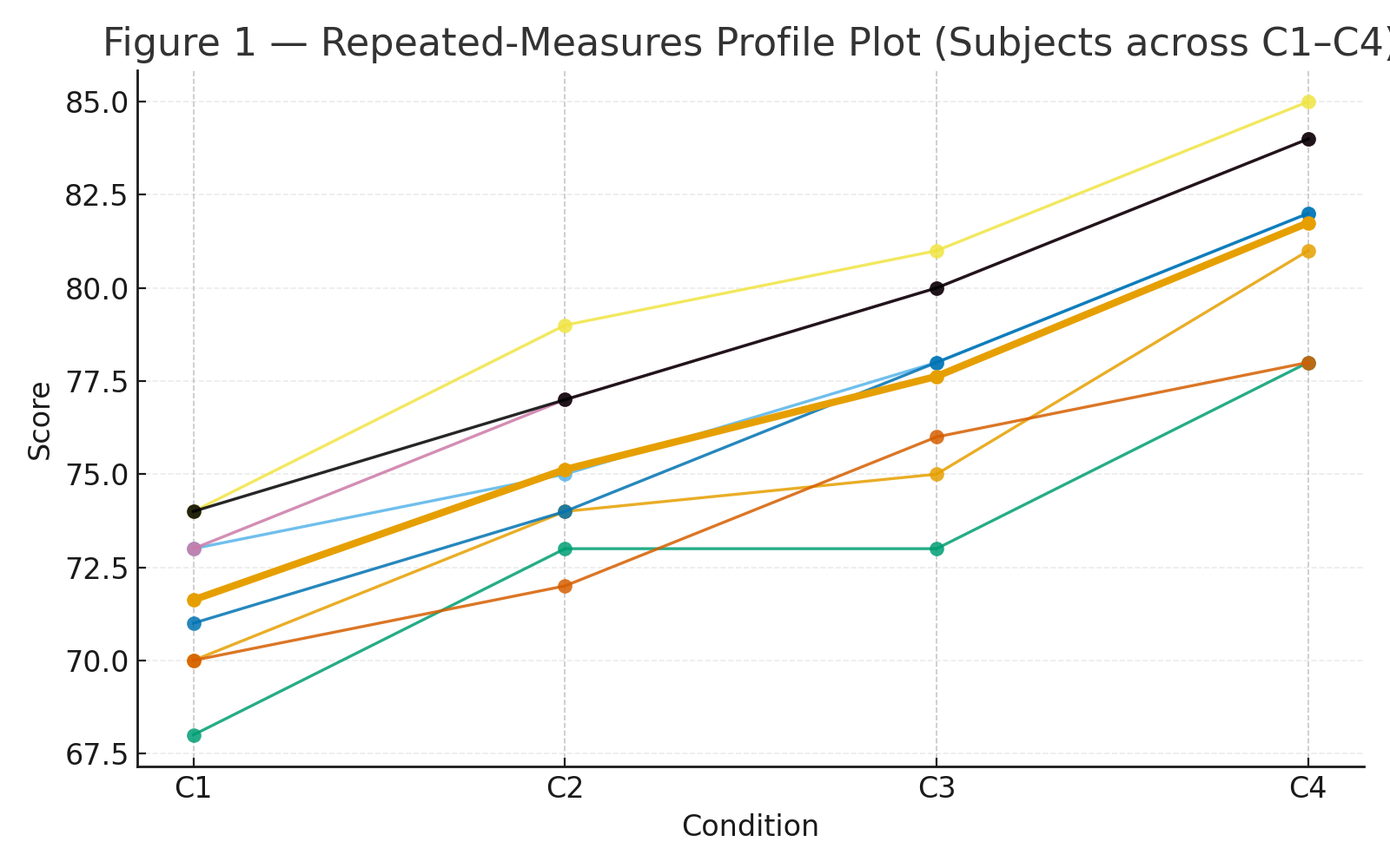
Figure 1: Profile plot (each subject as a line across the four conditions).

Data

Scores (rows = participants S1–S8; columns = conditions C1–C4):

Subject	C1	C2	C3	C4	Row sum	Row mean
S1	70	74	75	81	300	75.00
S2	73	75	78	82	308	77.00
S3	68	73	73	78	292	73.00
S4	74	79	81	85	319	79.75
S5	71	74	78	82	305	76.25
S6	70	72	76	78	296	74.00
S7	73	77	80	84	314	78.50
S8	74	77	80	84	315	78.75
Column sums	573	601	621	654	Grand sum = 2449	Grand mean \( \bar X = 2449/32 = 76.53125 \)

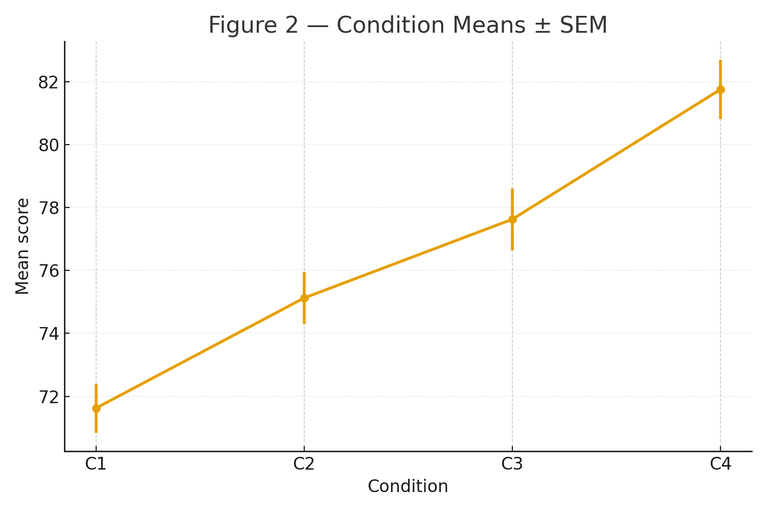
Figure 2: Means ± SEM for C1–C4 (bar/line).

Step 1 — Condition Means (and sample variances)

\[ \begin{aligned} \bar X_{\mathrm{C1}} &= 573/8 = 71.625, \quad & s^2_{\mathrm{C1}} &= 4.8393 \\ \bar X_{\mathrm{C2}} &= 601/8 = 75.125, \quad & s^2_{\mathrm{C2}} &= 5.5536 \\ \bar X_{\mathrm{C3}} &= 621/8 = 77.625, \quad & s^2_{\mathrm{C3}} &= 7.6964 \\ \bar X_{\mathrm{C4}} &= 654/8 = 81.750, \quad & s^2_{\mathrm{C4}} &= 7.0714 \end{aligned} \]

Step 2 — Sums of Squares

Notation: \(s=8\) subjects, \(k=4\) conditions, grand mean \( \bar X = 76.53125\).

2A. Total

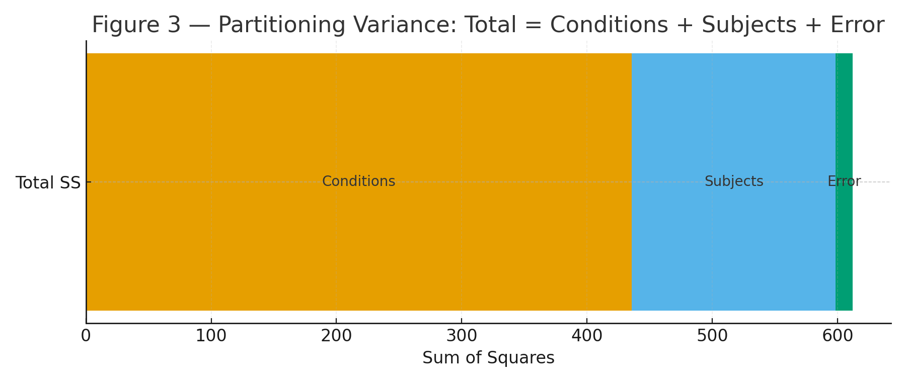
\[ SS_{\text{total}}=\sum_{i=1}^{s}\sum_{j=1}^{k}\bigl(X_{ij}-\bar X\bigr)^2 =\mathbf{611.96875}. \]

2B. Conditions (Treatment)

\[ SS_{\text{cond}}= s \sum_{j=1}^{k}\bigl(\bar X_{\cdot j}-\bar X\bigr)^2 = 8 \left[(71.625-76.53125)^2 + (75.125-76.53125)^2 + (77.625-76.53125)^2 + (81.75-76.53125)^2\right] =\mathbf{435.84375}. \]

2C. Subjects

\[ SS_{\text{subj}}= k \sum_{i=1}^{s}\bigl(\bar X_{i\cdot}-\bar X\bigr)^2 = 4 \sum_{i=1}^{8}\bigl(\bar X_{i\cdot}-76.53125\bigr)^2 =\mathbf{162.71875}. \]

2D. Error (Residual)

\[ SS_{\text{error}}= SS_{\text{total}} - SS_{\text{cond}} - SS_{\text{subj}} = 611.96875 - 435.84375 - 162.71875 =\mathbf{13.40625}. \]

Figure 3: Partitioning variance diagram (Total → Conditions + Subjects + Error).

Step 3 — Degrees of Freedom & Mean Squares

\[ \begin{aligned} df_{\text{cond}} &= k-1 = 3, \\ df_{\text{subj}} &= s-1 = 7, \\ df_{\text{error}} &= (s-1)(k-1) = 7\times3 = 21, \\ df_{\text{total}} &= sk-1 = 31. \end{aligned} \]

\[ MS_{\text{cond}} = \frac{SS_{\text{cond}}}{df_{\text{cond}}} =\frac{435.84375}{3}=\mathbf{145.28125},\qquad MS_{\text{error}} = \frac{SS_{\text{error}}}{df_{\text{error}}} =\frac{13.40625}{21}=\mathbf{0.6383928571}. \]

Step 4 — Test Statistic & p-value

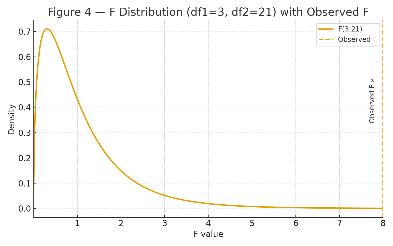
\[ F = \frac{MS_{\text{cond}}}{MS_{\text{error}}} = \frac{145.28125}{0.6383928571} =\mathbf{227.5734}. \] With \(df_1=3\) and \(df_2=21\), this is extremely large. The right-tail p-value is effectively \(p \lt 10^{-12}\) (i.e., \(p \ll .001\)).

Figure 4: F distribution with observed F marked and right-tail region shaded.

Repeated-Measures ANOVA Summary Table

Source	SS	df	MS	F	p
Conditions (within)	435.84375	3	145.28125	227.5734	< 1e-12
Subjects	162.71875	7	23.24554	—	—
Error (residual)	13.40625	21	0.63839	—	—
Total	611.96875	31	—	—	—

Interpretation

Mean performance increases steadily from C1 → C4, and the repeated-measures ANOVA shows a highly significant effect of Condition, \(F(3,21)=227.57,\, p\ll .001\). Follow-ups (e.g., paired t-tests with Bonferroni/Holm) can localize which pairs of conditions differ.

Assumptions (checklist)

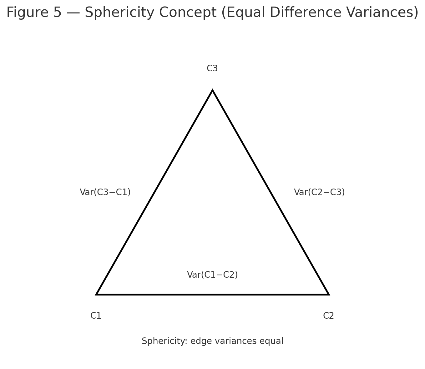
Sphericity (equal variances of the differences between condition pairs). If violated, apply Greenhouse–Geisser or Huynh–Feldt correction to \(df\).
Approximately normal scores within each condition.
No carryover/fatigue effects that confound order (counterbalancing helps).

Figure 5: Sphericity concept sketch (pairwise difference variances).

Practice self-test quiz

In the space below, please find practice problems and self-test quizzes. For full access, please signup free.