Lesson 18 — AI and Neural Networks (Intro)

Artificial intelligence (AI) develops systems that can produce predictions, classifications, or actions from data.
One powerful tool is the neural network, loosely inspired by simplified models of biological neurons.


From Statistics to AI

  • Regression predicts Y from X
  • Logistic regression predicts probability (0–1)
  • Neural networks generalize this idea: many inputs, many layers, nonlinear patterns

The Structure of a Neural Network

  1. Input layer — variables (X₁, X₂, …)
  2. Hidden layers — units that transform the input
  3. Output layer — prediction or classification

Each connection has a weight (like a slope in regression).


Formula for a Neuron

A single unit in the network:

$$z = \sum w_i X_i + b$$

$$y = f(z)$$

Where:

  • $$w_i$$ = weights
  • $$X_i$$ = inputs
  • $$b$$ = bias (like an intercept)
  • $$f(z)$$ = activation function (e.g., logistic, ReLU)

Learning in a Network

The network predicts outputs and compares them with the true answers.
The error is sent backward through the network to adjust weights.
This is called backpropagation.


Example

Predicting if a student will pass or fail based on:

  • Study hours
  • Attendance
  • Practice problems completed

Inputs → combined with weights → logistic activation → output: probability of passing.


Visuals
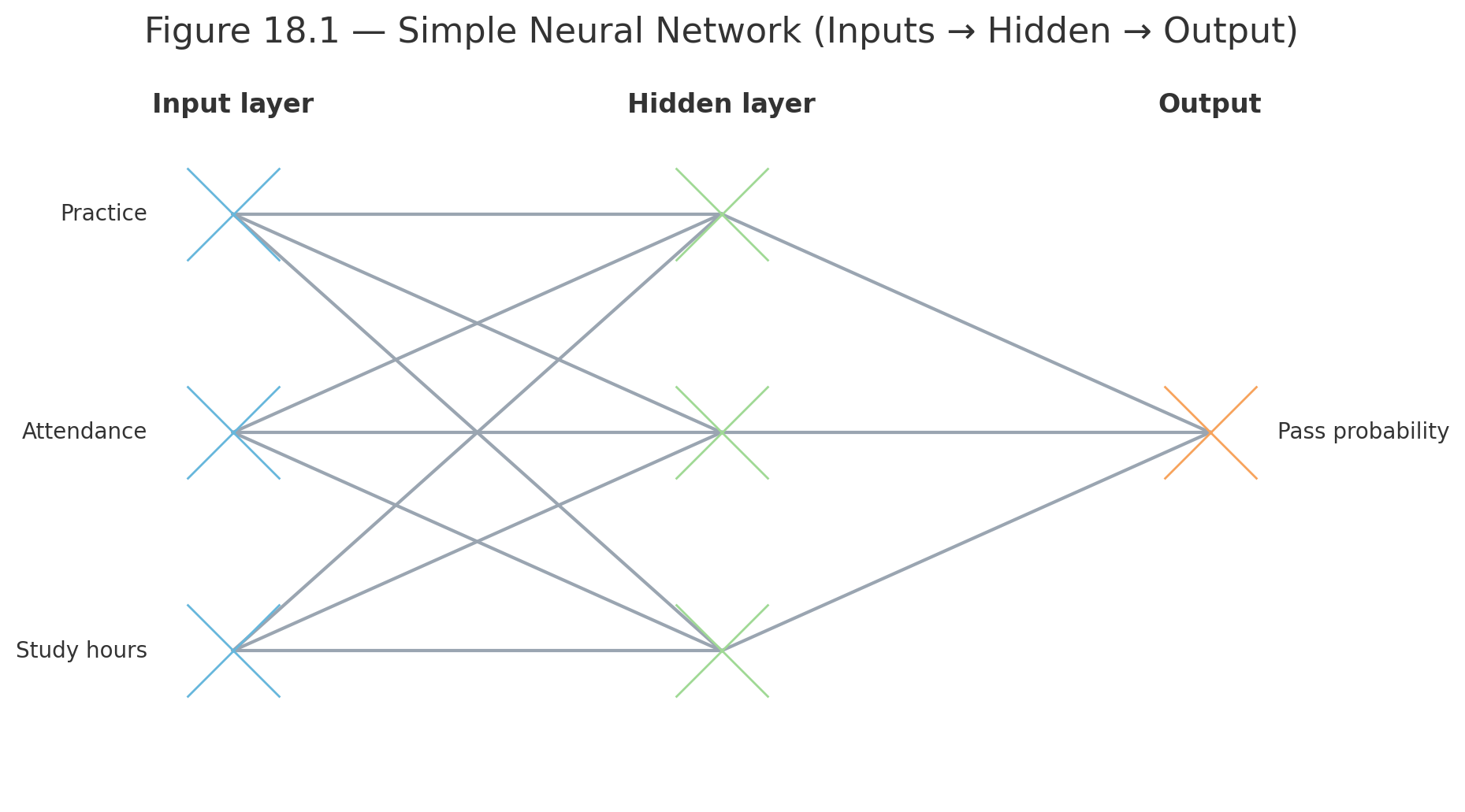
Simple neural network diagram

Figure 18.1 — Simple Neural Network (Inputs → Hidden → Output)
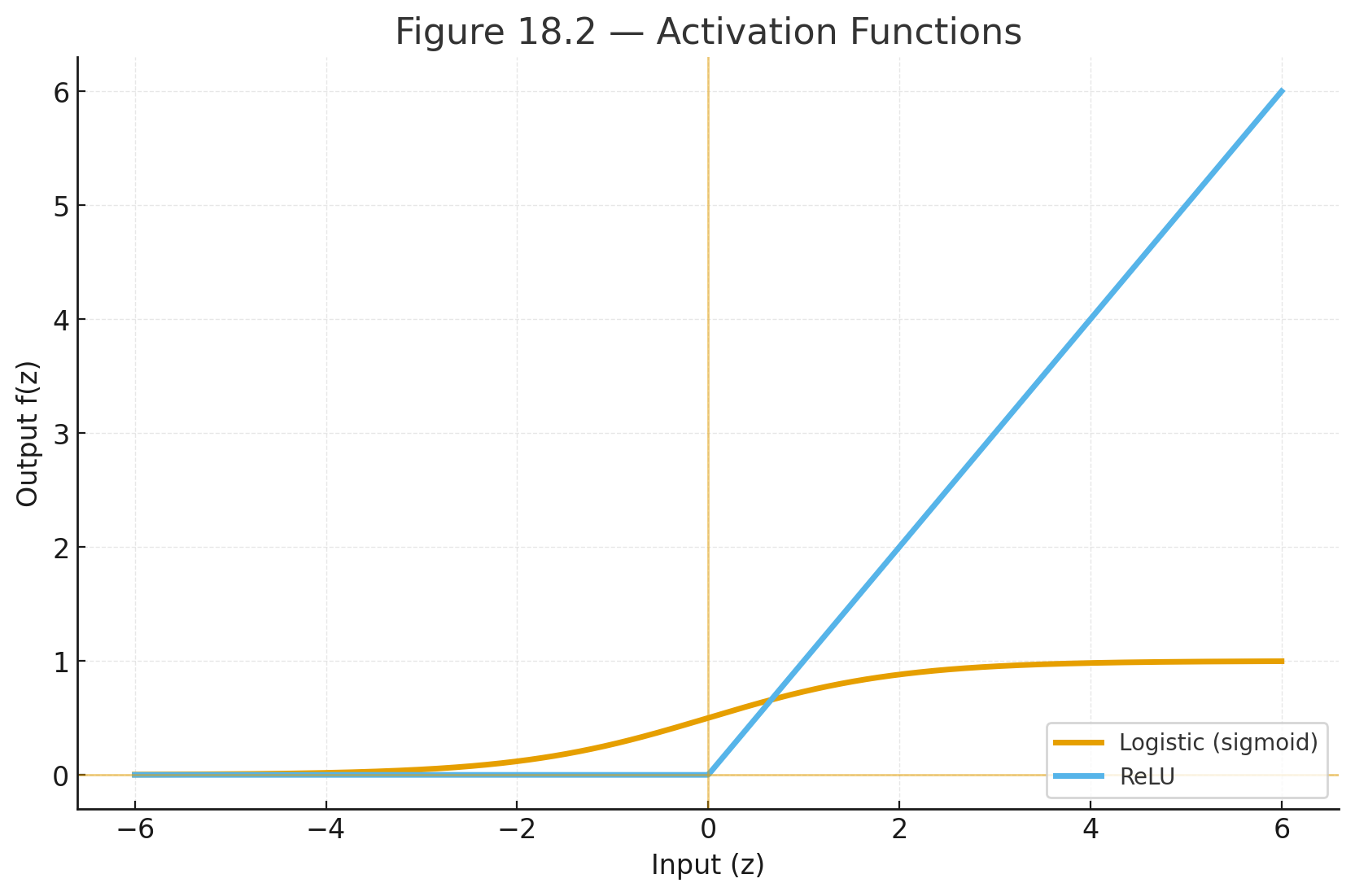
Activation functions: logistic and ReLU

Figure 18.2 — Activation Functions


Why This Matters

  • Neural networks can be viewed as extending regression and logistic regression.
  • They allow learning from large, complex datasets (images, speech, language).
  • Many modern AI systems, including translation, recognition, and chatbots, rely on neural-network models.

Practice self-test quiz

In the space below, please find practice problems and self-test quizzes. For full access, please signup free.
Lesson 17 — Regression Beyond the Line

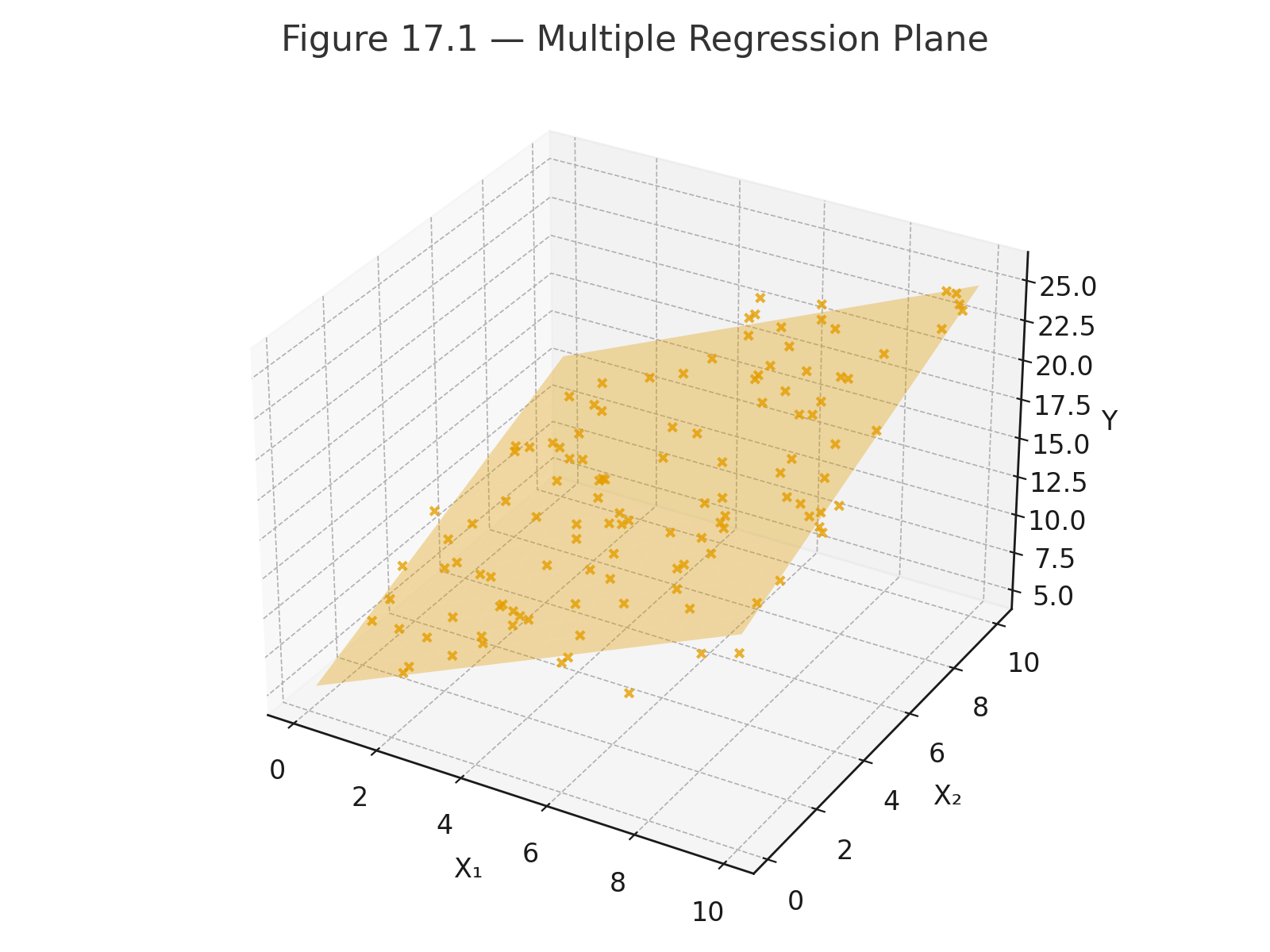
multiple regression plane
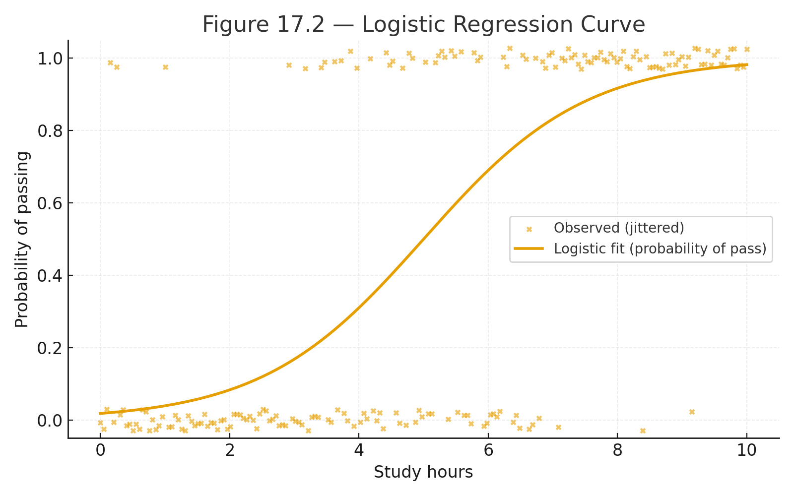
logistic curve

Simple regression predicts Y from one X.
But in real life, outcomes often depend on several variables — or may not be linear.

This chapter introduces multiple regression and logistic regression.


Multiple Regression

Formula:

$$\hat{Y} = a + b_1X_1 + b_2X_2 + \dots + b_kX_k$$

In words:
$$\text{Predicted Y} = \text{intercept} + (b_1 \times X_1) + (b_2 \times X_2) + \dots$$

Where:

  • $$X_1, X_2, \dots X_k$$ = predictors
  • $$b_1, b_2, \dots b_k$$ = slopes (weights for each predictor)

Example: Predicting college GPA from:

  • High school GPA ($$X_1$$)
  • Study hours ($$X_2$$)

Equation:
$$\hat{Y} = 1.0 + 0.5X_1 + 0.1X_2$$

Interpretation:

  • For each 1-point increase in HS GPA, college GPA rises 0.5.
  • For each extra study hour, GPA rises 0.1.

Coefficient of Determination

In multiple regression, $$R^2$$ tells us the proportion of variance explained by all predictors together.

Example: $$R^2 = 0.65$$ → predictors explain 65% of the outcome’s variability.


Logistic Regression

What if the outcome is yes/no (categorical)?
Example: Will a student pass or fail?

We use logistic regression.

Formula:

$$P(Y=1) = \frac{1}{1 + e^{-(a + bX)}}$$

In words:
$$\text{Probability of success} = \frac{1}{1 + e^{-(\text{intercept} + \text{slope} \times X)}}$$

Output: probability between 0 and 1.

Example: Predicting pass/fail from study hours.

  • Equation: $$P = \frac{1}{1 + e^{-( -2 + 0.5X )}}$$
  • If X = 6 hours: $$P = \frac{1}{1 + e^{-1}} = 0.73$$
  • About 73% chance of passing.

Visuals

Figure 17.1 — Multiple regression plane: Y predicted from two predictors.

Figure 17.2 — Logistic regression curve: probability vs. study hours.


Why This Matters

  • Multiple regression = prediction with many factors
  • Logistic regression = prediction when the outcome is categorical
  • $$R^2$$ = strength of prediction

These methods expand the power of regression beyond a straight line, preparing for modern predictive modeling.

Practice self-test quiz

In the space below, please find practice problems and self-test quizzes. For full access, please signup free.
Lesson 16 — Machine Learning Basics

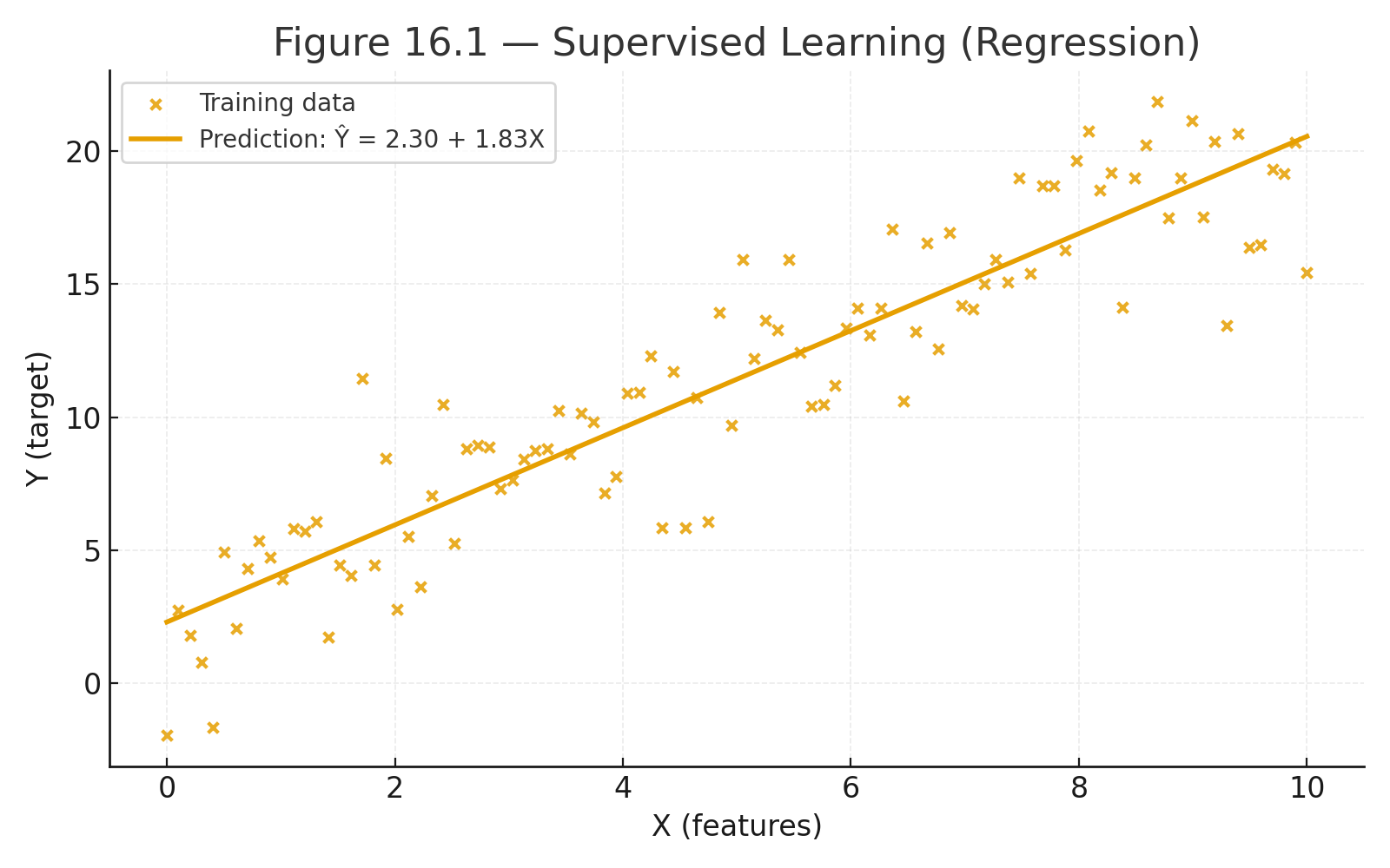
supervised regression
unsupervised k means
overfitting vs generalization

Machine learning is where statistics meets computers.
Instead of only writing formulas, we teach a computer to learn patterns from data.


What is Machine Learning?

Machine learning uses algorithms to improve automatically with experience.

  • Supervised learning: the computer is given examples with correct answers.
  • Unsupervised learning: the computer finds patterns without answers.

Supervised Learning

Goal: predict Y from X.

Examples:

  • Predict exam scores from study hours
  • Predict house price from size, location, and age

Steps:

  1. Split data into training set and test set
  2. Train the model on training data
  3. Test accuracy on new (unseen) data

Formula (simple linear regression as machine learning):
$$\hat{Y} = a + bX$$

Here, the computer “learns” $$a$$ and $$b$$ from the data.


Unsupervised Learning

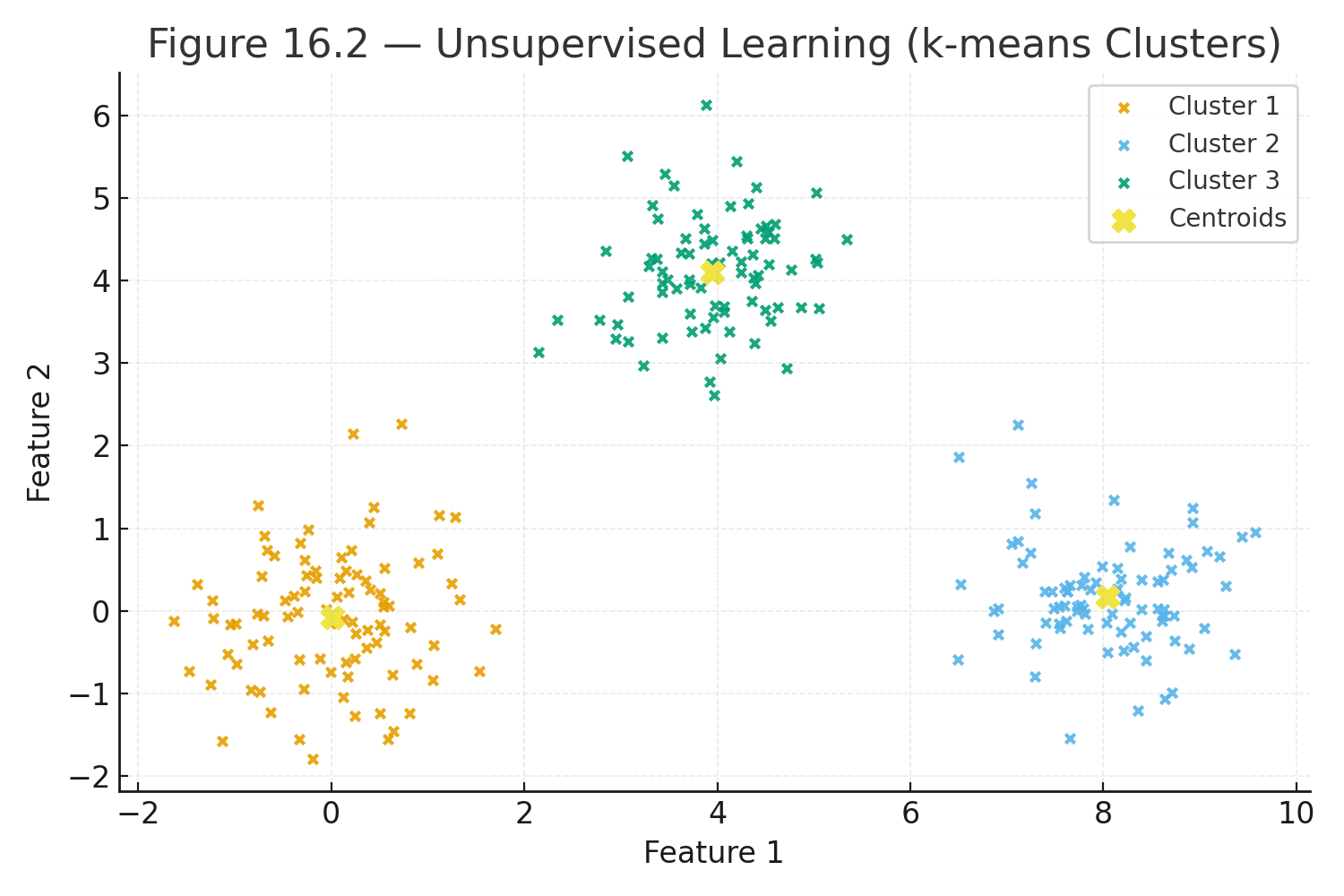
Goal: find hidden structure in the data.

Examples:

  • Group students by study habits
  • Cluster shoppers by buying patterns

Algorithms:

  • k-means clustering
  • Hierarchical clustering

No “correct answer” is given — the computer organizes the data.


Overfitting vs. Generalization

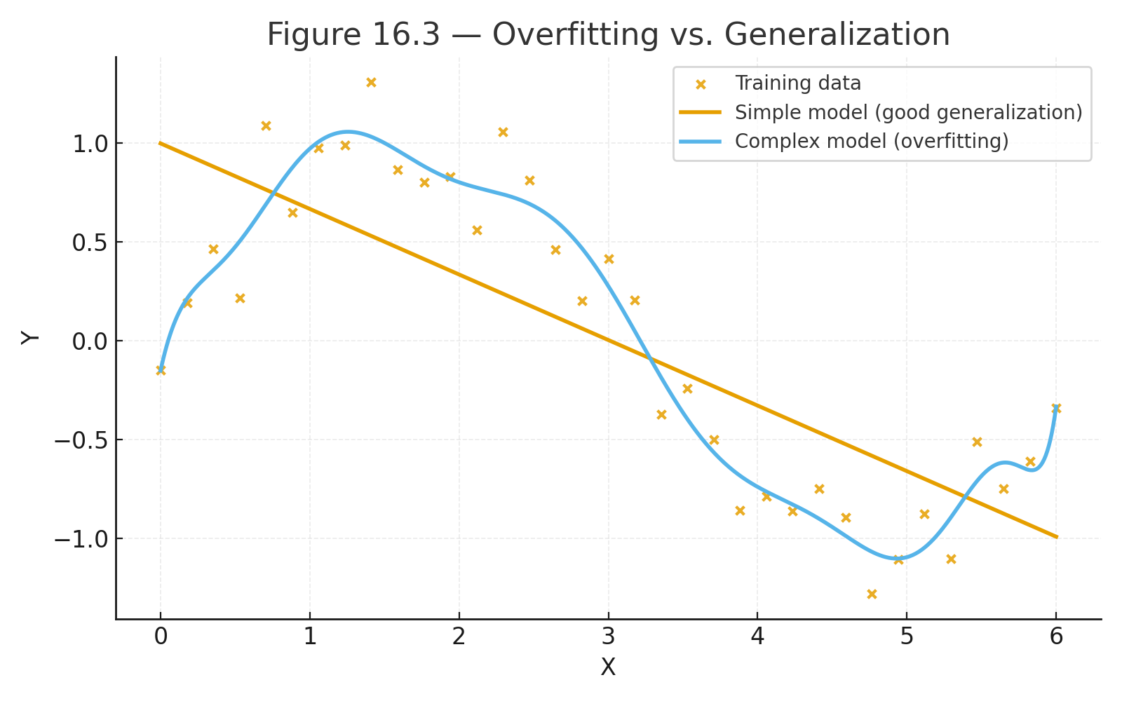
  • Overfitting: the model memorizes the training data but fails on new data.
  • Generalization: the model maintains useful predictive performance on new data.

Example:
If a student memorizes past exam answers (overfit), they may fail a new test.
If they learn the concepts (generalize), they are more likely to succeed.


Key Concepts

  • Training set: data used to build the model
  • Test set: data used to evaluate performance
  • Accuracy: how well the model predicts new data

Visuals

Figure 16.1 — Supervised learning example: regression line predicting Y from X.

Figure 16.2 — Unsupervised learning example: scatterplot with clusters (k-means).

Figure 16.3 — Overfitting vs. generalization: wiggly curve vs. smooth line.


Why This Matters

Machine learning grows directly out of statistics:

  • Regression → prediction
  • ANOVA → comparison of group means
  • Clustering → organizing data

By learning the basics of ML, students see how statistical ideas contribute to AI.

Practice self-test quiz

In the space below, please find practice problems and self-test quizzes. For full access, please signup free.
Lesson 15 — Resampling and Simulation

bootstrap
bootstrap randomization
monte carlo

Classical statistics uses formulas and tables.
Modern computing gives us another way: resampling and simulation.

Instead of relying only on theory, we let the computer generate thousands of samples and see what happens.


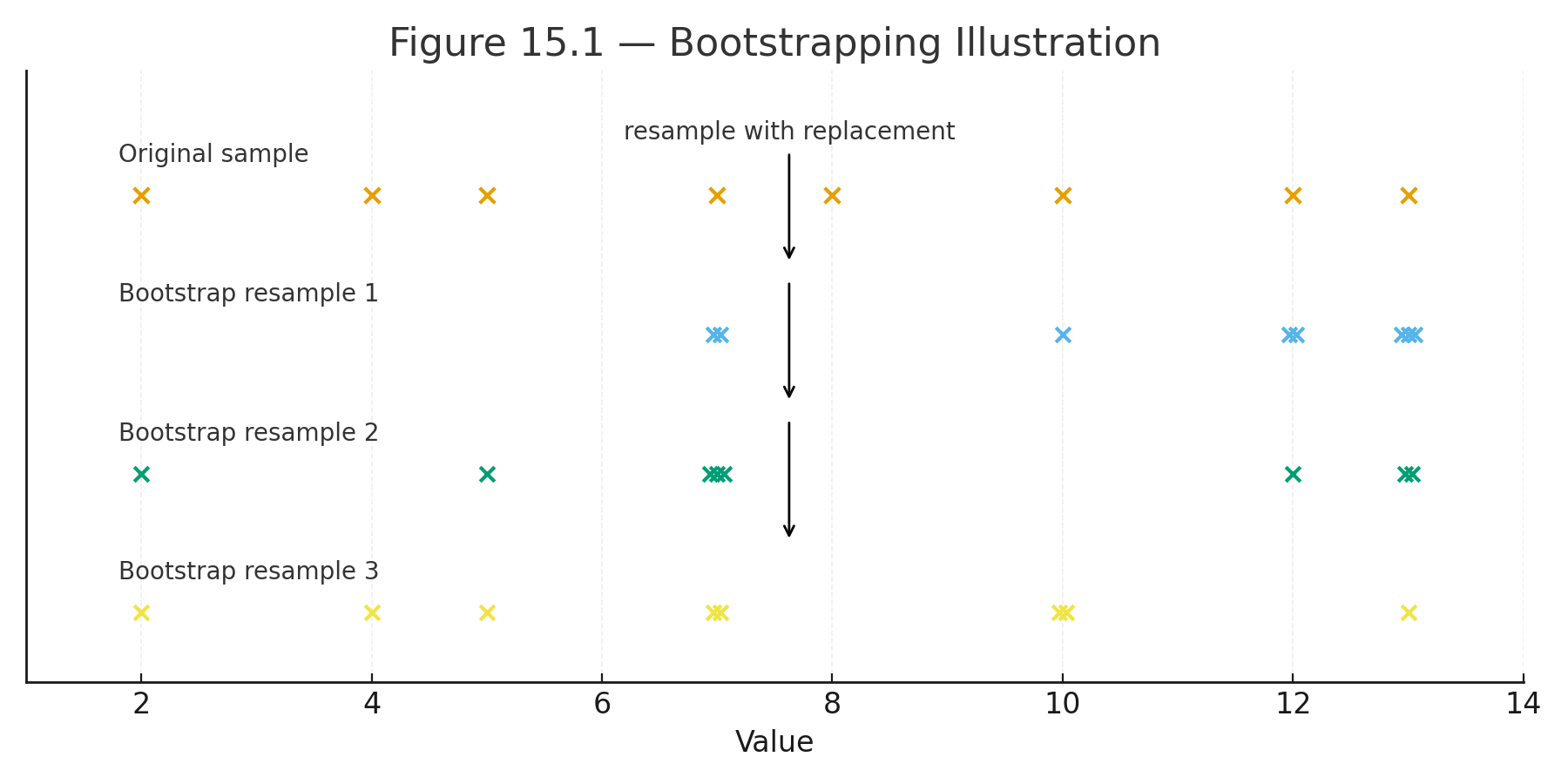
Bootstrapping

Bootstrapping means resampling with replacement from the original data.

Steps:

  1. Take a sample of size $$n$$ from the data (with replacement).
  2. Compute the statistic (mean, median, correlation).
  3. Repeat thousands of times.
  4. Use the distribution of resampled statistics to estimate confidence intervals.

Example:
Data = [5, 6, 7, 9].
Resample 1000 times, compute mean each time.
The distribution of means gives an estimate of the true mean’s variability.


Randomization (Permutation) Tests

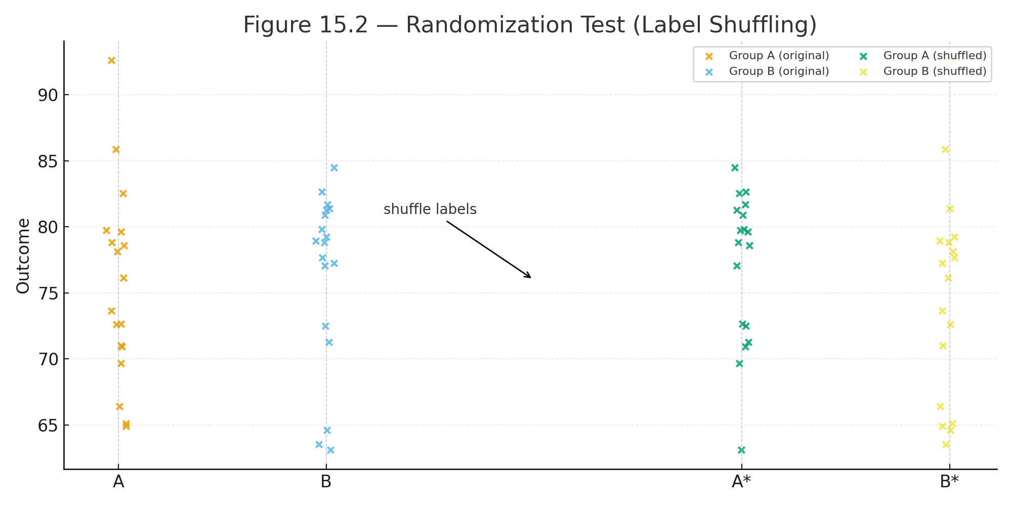
Used to test hypotheses by shuffling labels.

Steps:

  1. Combine all data.
  2. Randomly assign to groups.
  3. Compute the difference in means.
  4. Repeat thousands of times.
  5. Compare the observed difference to this distribution.

This shows whether the observed effect could be due to chance.


Monte Carlo Simulation

Monte Carlo methods use random numbers to model complex processes.

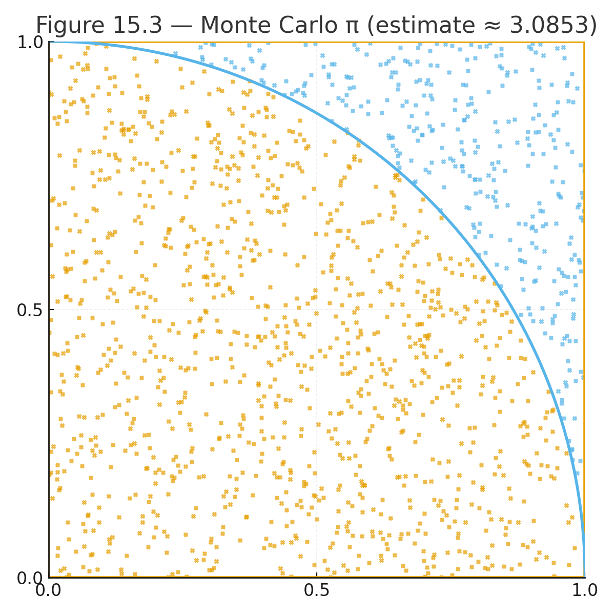
Example: Estimating $$\pi$$.

  • Randomly throw points into a square.
  • Count how many fall inside the circle quarter.
  • $$\pi \approx 4 \times \tfrac{\text{inside circle}}{\text{total points}}$$.

Why Resampling Works

Resampling uses the data itself as a model of the population.
It avoids assumptions (like normality) and adapts to modern computing power.


Visuals

Figure 15.1 — Bootstrapping illustration: resampling from a small dataset with replacement.

Figure 15.2 — Randomization test: labels shuffled between groups.

Figure 15.3 — Monte Carlo: random points filling a square and a quarter circle.


Why This Matters

Resampling and simulation show students that statistics is not only about formulas.
Computers allow us to see probability in action.
This approach prepares students for data science, where simulation is as important as theory.

Practice self-test quiz

In the space below, please find practice problems and self-test quizzes. For full access, please signup free.
Lesson 14 — Big Data

big data

In the past, statistics often dealt with comparatively small datasets: 20 students in a class, 50 patients in a trial.
Today, we live in the age of big data: millions of tweets, billions of web pages, streams of data from phones, sensors, and satellites.

Big data changes the scale of statistics.


What is Big Data?

Big data is often described by the 3 Vs:

  1. Volume — enormous amounts of data (terabytes, petabytes)
  2. Velocity — data generated quickly (social media streams, stock markets)
  3. Variety — many forms (numbers, text, images, audio, video)

Sometimes a fourth V is added: Veracity (how reliable are the data?).


Why Big Data Matters

  • Many classical methods are introduced using small, relatively clean teaching datasets.
  • With big data, we need algorithms and computers to process information.
  • Sampling error may be reduced when a well-defined finite population is fully observed, although coverage, measurement, selection, and generalization problems remain.
  • Visualization and summaries are critical to make sense of huge datasets.

Example

  • A teacher records grades for 30 students → small dataset.
  • YouTube collects billions of video views per day → big data.

Some familiar statistical tools remain useful (mean, median, regression), but the scale requires computational methods.


Tools for Big Data

  • Databases (SQL, NoSQL) to store data
  • Distributed computing (Hadoop, Spark) to process data
  • Statistical programming (R, Python) for analysis

Visuals

Figure 14.1 — Big Data and the 3 Vs. Diagram showing Volume, Velocity, Variety (and Veracity) in overlapping circles.


Why This Matters

Big data connects statistics to the modern world:

  • Online behavior, medical records, GPS signals, shopping patterns
  • Algorithms can identify patterns in datasets too large for manual inspection
  • Large datasets support many modern AI and machine-learning systems

Practice self-test quiz

In the space below, please find practice problems and self-test quizzes. For full access, please signup free.
Part 6 — Modern Statistics: Data, AI, and Machine Learning

Welcome to Part 6 — Modern Statistics: Data, AI, and Machine Learning of this free online high school statistics textbook. This forward-looking section introduces high school students to the exciting intersection of traditional statistics with modern data science, artificial intelligence, and machine learning concepts. Through accessible explanations, real-world examples, and intuitive labs, learners explore big data handling, basic machine learning algorithms, predictive modeling, ethical considerations in AI, and how statistical principles underpin today's data-driven technologies—all tailored for pre-college preparation and AP Statistics extensions.

Perfect for students curious about data science, machine learning basics, and AI applications, Part 6 builds on foundational statistics to show real-world relevance in fields like technology, healthcare, and business, with hands-on activities and clear connections to classical methods.

Lessons in Part 6: Modern Statistics

  1. Lesson 14 — Big Data
  2. Lesson 15 — Resampling and Simulation
  3. Lesson 16 — Machine Learning Basics
  4. Lesson 17 — Regression Beyond the Line
  5. Lesson 18 — AI and Neural Networks (Intro)
  6. Lesson 19 — Ethics in Data and AI

Lesson 13 — Degrees of Freedom Cookbook

Every statistical test requires degrees of freedom (df).
Degrees of freedom tell us how many independent pieces of information are available once totals or means are fixed.
They determine which row of the t-table or F-table we use.

General rule:

$$df = \text{number of observations} - \text{number of constraints}$$


t-tests

  • One-sample t-test:
    $$df = n - 1$$
  • Independent-samples t-test:
    $$df = n_1 + n_2 - 2$$
  • Paired-samples t-test:
    $$df = n - 1$$

One-way ANOVA

  • Between groups:
    $$df_{\text{between}} = k - 1$$
  • Within groups:
    $$df_{\text{within}} = N - k$$
  • Total:
    $$df_{\text{total}} = N - 1$$

Where $$k$$ = number of groups, $$N$$ = total number of scores.


Factorial ANOVA (2 × 2 Example)

  • Factor A: $$df_A = a - 1$$
  • Factor B: $$df_B = b - 1$$
  • Interaction: $$df_{A \times B} = (a-1)(b-1)$$
  • Error: $$df_{\text{within}} = N - ab$$

Repeated-Measures ANOVA

  • Rows (subjects): $$df_{\text{rows}} = n - 1$$
  • Columns (conditions): $$df_{\text{columns}} = k - 1$$
  • Error: $$df_{\text{error}} = (n - 1)(k - 1)$$

Where $$n$$ = number of subjects, $$k$$ = number of conditions.


Mixed (Split-Plot) ANOVA

  • Between factor: $$df_{\text{between}} = a - 1$$
  • Subjects within groups: $$df_{\text{subjects}} = N - a$$
  • Within factor: $$df_{\text{within}} = b - 1$$
  • Interaction: $$df_{A \times B} = (a-1)(b-1)$$

Chi-square

  • Goodness-of-fit: $$df = k - 1$$
  • Independence: $$df = (r - 1)(c - 1)$$

Where $$k$$ = number of categories, $$r$$ = rows, $$c$$ = columns.


Visuals

Degrees of Freedom — Quick Cookbook
Test / Designdf formulaNotes
One-sample t-test\( df = n - 1 \)Single group vs. constant.
Independent-samples t-test\( df = n_1 + n_2 - 2 \)Equal-variance (pooled) case.
Paired-samples t-test\( df = n - 1 \)Based on the \( n \) differences.
One-way ANOVA — Between\( df_{\text{between}} = k - 1 \)\( k \) groups.
One-way ANOVA — Within (Error)\( df_{\text{within}} = N - k \)\( N \) total scores.
One-way ANOVA — Total\( df_{\text{total}} = N - 1 \)Sum of between + within df.
Factorial ANOVA — Factor A\( df_A = a - 1 \)\( a \) levels of A.
Factorial ANOVA — Factor B\( df_B = b - 1 \)\( b \) levels of B.
Factorial ANOVA — Interaction\( df_{A\times B} = (a-1)(b-1) \)Interaction A×B.
Factorial ANOVA — Error (Within)\( df_{\text{within}} = N - ab \)\( ab \) cells total.
Repeated-measures ANOVA — Subjects (Rows)\( df_{\text{rows}} = n - 1 \)\( n \) subjects.
Repeated-measures ANOVA — Conditions (Columns)\( df_{\text{columns}} = k - 1 \)\( k \) conditions.
Repeated-measures ANOVA — Error\( df_{\text{error}} = (n - 1)(k - 1) \)Subjects × conditions.
Mixed (Split-Plot) ANOVA — Between factor\( df_{\text{between}} = a - 1 \)\( a \) groups (between-subjects).
Mixed (Split-Plot) ANOVA — Subjects within groups\( df_{\text{subjects}} = N - a \)\( N \) subjects total.
Mixed (Split-Plot) ANOVA — Within factor\( df_{\text{within}} = b - 1 \)\( b \) repeated levels.
Mixed (Split-Plot) ANOVA — Interaction\( df_{A\times B} = (a-1)(b-1) \)Between × within.
Chi-square — Goodness-of-fit\( df = k - 1 \)\( k \) categories.
Chi-square — Independence\( df = (r - 1)(c - 1) \)\( r \) rows, \( c \) columns.

Variables: \( n \)=sample size, \( n_1,n_2 \)=group sizes, \( N \)=total scores, \( k \)=# of groups/conditions, \( a,b \)=levels of factors A,B, \( r,c \)=rows, columns.


Why This Matters

Degrees of freedom link sample size to critical values.
They tell us how much room for variability exists in the data.
With this quick cookbook, you can locate the right df for any test.

Practice self-test quiz

In the space below, please find practice problems and self-test quizzes. For full access, please signup free.
Lesson 12 — Chi-square Tests

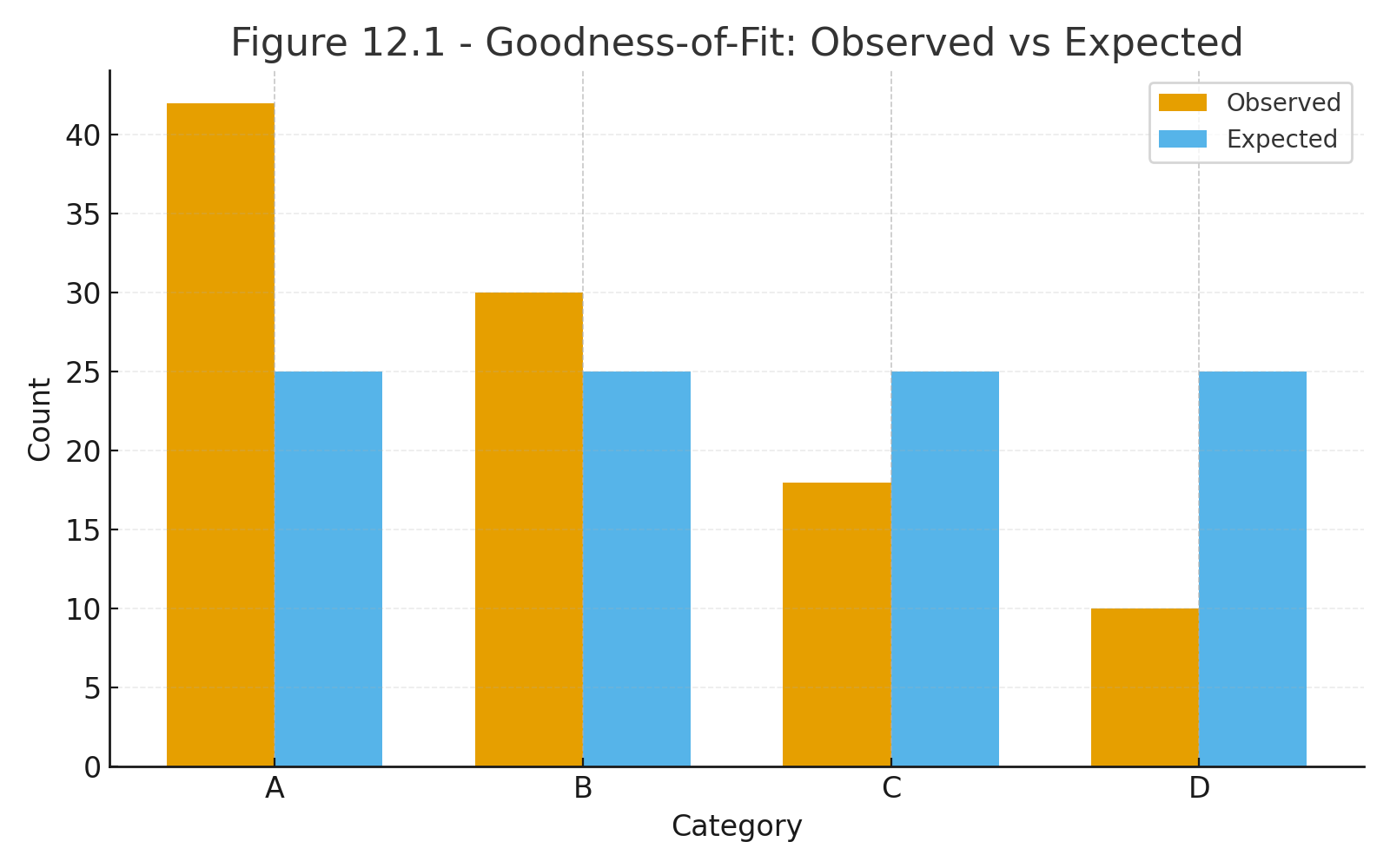
gof observed expectancies
independence 2x2
phi cramer

The chi-square test ($$\chi^2$$) is used with categorical (nominal) data.
It compares observed frequencies with expected frequencies.


Chi-square Goodness-of-Fit

When to Use:

  • One categorical variable
  • Test if observed frequencies match expected frequencies

Formula:
$$\chi^2 = \sum \frac{(O - E)^2}{E}$$

In words:
$$\chi^2 = \text{sum of squared differences between observed and expected, divided by expected}$$

Example:
Survey of favorite subjects (Math, Science, English).
Expected = equal (⅓ each), Observed = [25, 30, 45].
Compute each (O–E)²/E, sum = χ².


Chi-square Test of Independence

When to Use:

  • Two categorical variables
  • Test whether they are associated (independent or not)

Formula:
$$\chi^2 = \sum \frac{(O - E)^2}{E}$$

Where expected frequencies:
$$E = \frac{(\text{row total})(\text{column total})}{\text{grand total}}$$

Example:
Gender (Male/Female) × Sport (Soccer/Basketball/Tennis).
If observed counts differ from expected, χ² tests independence.


Chi-square Correlation Measures

Chi-square can also give a measure of association strength between categorical variables.

  • Phi coefficient (φ): for 2 × 2 tables

$$\phi = \sqrt{\frac{\chi^2}{N}}$$

  • Cramer’s V: for larger tables

$$V = \sqrt{\frac{\chi^2}{N(k-1)}}$$

Where $$k = \min(\text{rows}, \text{columns})$$.

  • Contingency coefficient (C):

$$C = \sqrt{\frac{\chi^2}{\chi^2 + N}}$$


Example (Phi, Cramer’s V, Contingency C)

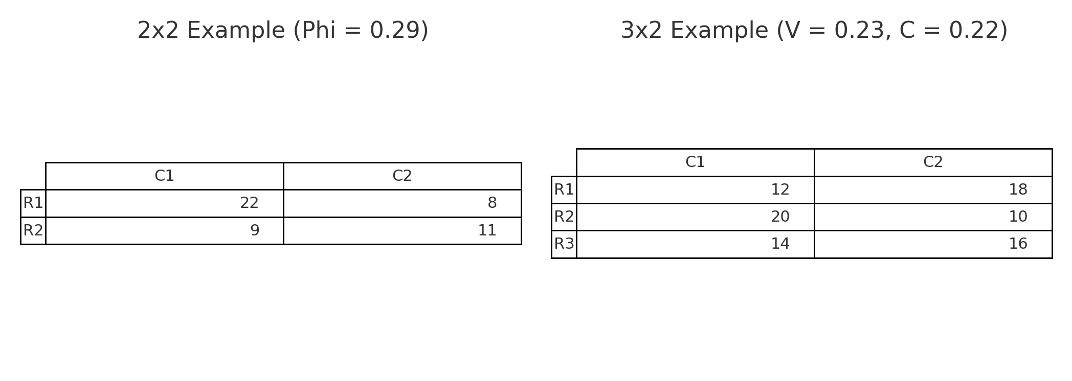
Suppose χ² = 10.0, N = 100.

  • For 2 × 2: $$\phi = \sqrt{10/100} = \sqrt{0.1} = 0.32$$
  • For 3 × 2 table: $$V = \sqrt{10/(100(2-1))} = \sqrt{0.1} = 0.32$$
  • Contingency coefficient: $$C = \sqrt{10/(10+100)} = \sqrt{0.09} = 0.30$$

Definition

  • Goodness-of-fit: one categorical variable vs. expected distribution
  • Independence: relationship between two categorical variables
  • Correlation measures: strength of association in categorical tables (φ, V, C)

Visuals

Figure 12.1 — Goodness-of-fit example: observed vs. expected bar chart.

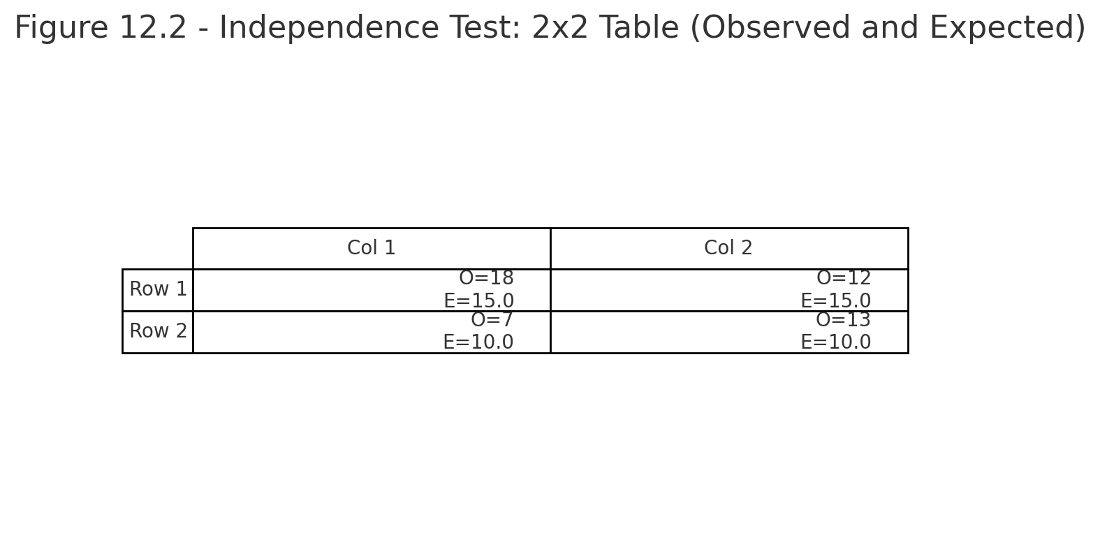
Figure 12.2 — Independence test: 2 × 2 contingency table with expected values.

Figure 12.3 — Phi, Cramer’s V, and C illustrated with 2 × 2 and 3 × 2 tables.


Why This Matters

Chi-square lets us analyze data that are counts rather than scores.
It extends statistical testing beyond numbers into categories — essential for psychology, sociology, education, and medicine.

Practice self-test quiz

In the space below, please find practice problems and self-test quizzes. For full access, please signup free.
Lesson 11 — Non-parametric Tests

mann whitney
wilcoxon test
kruskal wallis test
friedman test

Most tests so far (t-tests, ANOVA, regression) are parametric.
They assume:

  • Interval/ratio data
  • Approximately normal distribution
  • Homogeneity of variance

But what if these assumptions are not met?
Or if data are ranks or categories?

Then we use non-parametric tests.
They make fewer assumptions and are based on ranks, not raw scores.


Mann–Whitney U Test

When to Use:

  • Compare two independent groups, ordinal or non-normal data.
  • Non-parametric alternative to independent t-test.

Formula:
$$U = n_1 n_2 + \frac{n_1(n_1 + 1)}{2} - R_1$$

Where $$R_1$$ = sum of ranks for group 1.

Example:
Two groups (n = 5 each) ranked by performance. Compute rank sums, plug into U formula.


Wilcoxon Signed-Rank Test

When to Use:

  • Compare the same group measured twice.
  • Ordinal or non-normal data.
  • Non-parametric alternative to paired t-test.

Procedure:

  1. Compute differences (After – Before).
  2. Rank absolute differences.
  3. Add signs.
  4. Test statistic = smaller signed sum.

Example:
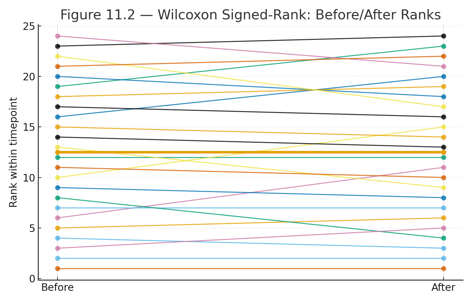
5 students tested before/after training → positive ranks dominate → training helps.


Kruskal–Wallis Test

When to Use:

  • Compare 3+ independent groups.
  • Ordinal or non-normal data.
  • Non-parametric alternative to one-way ANOVA.

Formula:
$$H = \frac{12}{N(N+1)} \sum \frac{R_j^2}{n_j} - 3(N+1)$$

Where:

  • $$R_j$$ = sum of ranks in group j
  • $$n_j$$ = group size
  • $$N$$ = total number of cases

Example:
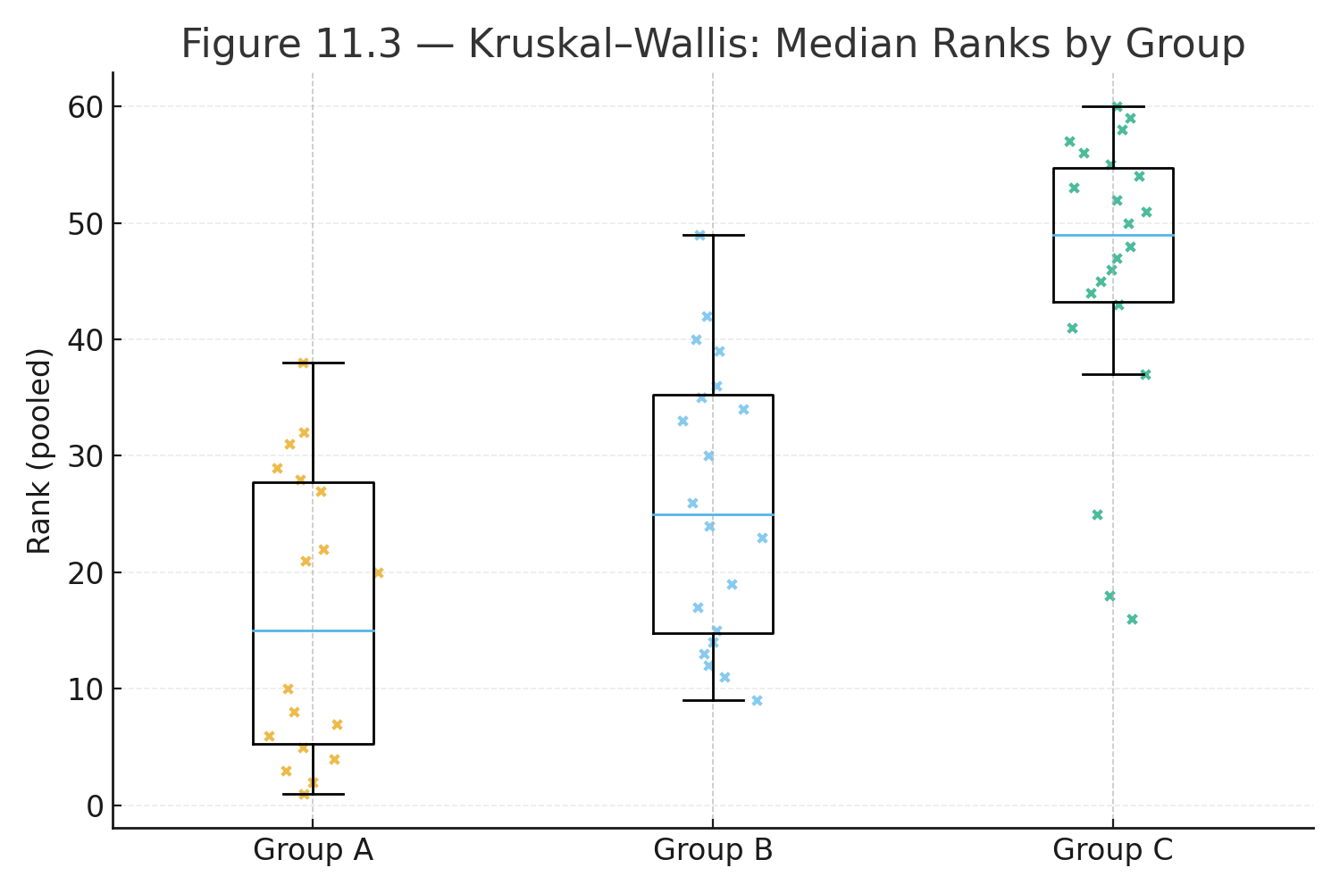
Three therapy groups (n = 6 each). Rank improvement scores → compare H to χ² distribution.


Friedman Test

When to Use:

  • Compare 3+ related groups (repeated measures).
  • Ordinal or non-normal data.
  • Non-parametric alternative to repeated-measures ANOVA.

Formula:
$$Q = \frac{12}{nk(k+1)} \sum R_j^2 - 3n(k+1)$$

Where:

  • $$R_j$$ = rank sum for each condition
  • $$n$$ = number of subjects
  • $$k$$ = number of conditions

Example:
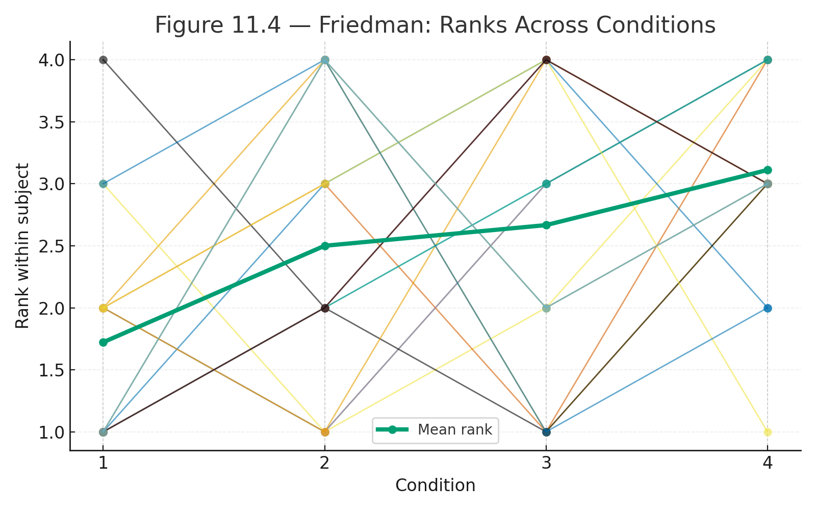
10 participants ranked across 3 learning tasks. Compare Q to χ² distribution.


Definition

  • Non-parametric tests: statistical tests based on ranks, not raw scores
  • Used when parametric assumptions fail or data are ordinal

Visuals

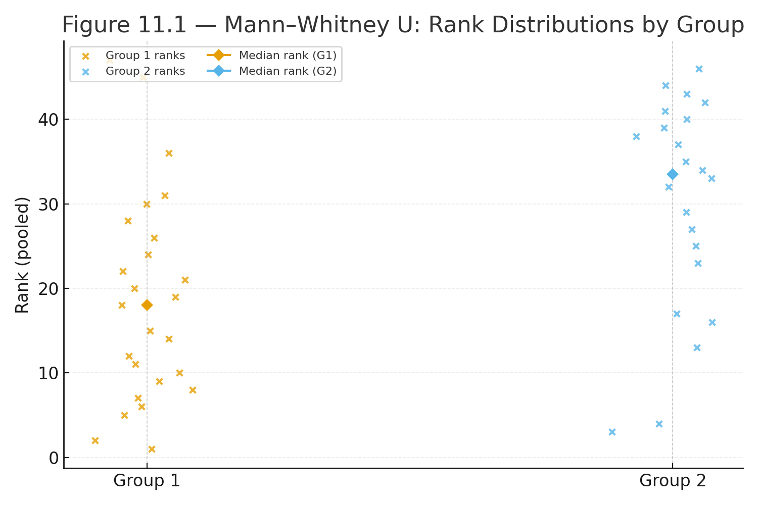
Figure 11.1 — Mann–Whitney U test: two groups compared by rank distributions.

Figure 11.2 — Wilcoxon signed-rank: before/after ranks with arrows.

Figure 11.3 — Kruskal–Wallis layout: three groups compared by median ranks.

Figure 11.4 — Friedman layout: subjects compared across repeated conditions.


Why This Matters

Non-parametric tests give us flexibility.
They extend statistical reasoning to real-world data that are messy, skewed, or categorical.
They are essential tools for psychology, education, and biology.

Practice self-test quiz

In the space below, please find practice problems and self-test quizzes. For full access, please signup free.

Lesson 10 — Regression

scatter intercept
slope intercept

Correlation tells us the strength of the relationship between two variables.
Regression goes one step further: it gives us an equation to predict one variable from another.


The Regression Equation

The regression line predicts Y from X.

Symbolic formula:
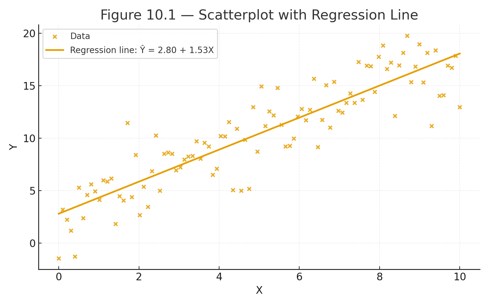
$$\hat{Y} = a + bX$$

Formula in words:
$$\text{Predicted Y} = \text{intercept} + (\text{slope} \times X)$$

Where:

  • $$\hat{Y}$$ = predicted value of Y
  • $$a$$ = intercept (value of Y when X = 0)
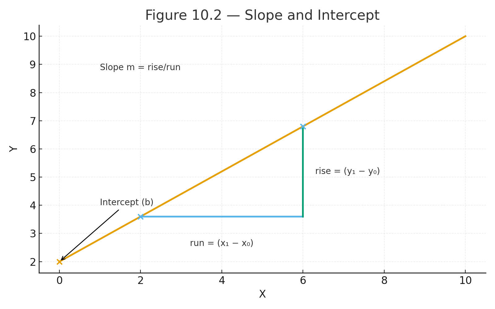
  • $$b$$ = slope (change in Y for each 1-unit change in X)

Slope and Intercept

The slope is calculated as:

$$b = \frac{\sum (X - \bar{X})(Y - \bar{Y})}{\sum (X - \bar{X})^2}$$

The intercept is:

$$a = \bar{Y} - b\bar{X}$$


Example

Study hours (X) and test scores (Y):

  • X = [2, 4, 6]
  • Y = [50, 60, 80]
  • $$\bar{X} = 4, \quad \bar{Y} = 63.3$$

Step 1: Slope

  • Numerator = Σ(X – X̄)(Y – Ȳ) = 60
  • Denominator = Σ(X – X̄)² = 8
  • $$b = \tfrac{60}{8} = 7.5$$

Step 2: Intercept

  • $$a = 63.3 - (7.5)(4) = 33.3$$

Regression equation:
$$\hat{Y} = 33.3 + 7.5X$$

Interpretation: each extra study hour adds about 7.5 points to the predicted test score.


Coefficient of Determination

The square of the correlation, $$r^2$$, shows the proportion of variance explained by regression.

Here: $$r^2 = 0.9643$$, so about 96.4% of score variation is explained by study hours.


Definition

  • Regression: predicts one variable from another using a line
  • Slope (b): how much Y changes per unit change in X
  • Intercept (a): expected value of Y when X = 0
  • r²: proportion of variance explained by regression

Visuals

Figure 10.1 — Scatterplot with regression line (Y predicted from X).

Figure 10.2 — Illustration of slope (rise/run) and intercept.


Why This Matters

Regression is a predictive tool.
It connects statistical description to practical forecasting: how much outcome (Y) changes with predictor (X).
It is the basis for more advanced models used in science, business, and data analysis.

Practice self-test quiz

In the space below, please find practice problems and self-test quizzes. For full access, please signup free.