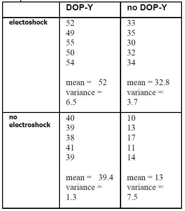
Story 17 — Example of a 2x3 factorial experiment

The layout of a 2x3 factorial ANOVA


B1

B2

B3


A1

A1B1
Subject 1
Subject 2
Subject 3
Subject 4
Subject 5

A1B2
Subject 6
Subject 7
Subject 8
Subject 9
Subject 10

A1B3
Subject 11
Subject 12
Subject 13
Subject 14
Subject 15


A2

A2B1
Subject 16
Subject 17
Subject 18
Subject 19
Subject 20

A2B2
Subject 21
Subject 22
Subject 23
Subject 24
Subject 25

A2B3
Subject 26
Subject 27
Subject 28
Subject 29
Subject 30


In this example of a factorial design, we have a 2x3 (we read this as "a two by three") factorial. Two by three, meaning two factors: A and B. "two" meaning two levels for factor A. "three" meaning three levels for B. In another case of a 3x2 factorial design we have two factors, A and B, factor A three levels, factor B two levels.


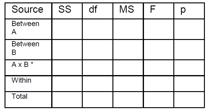
FORMAT OF 2x3 FACTORIAL ANOVA SUMMARY TABLE

Source

SS

df

MS

F

p

Between A


Between B


AxB (interaction)


Within


Total


Interaction -factorial designs

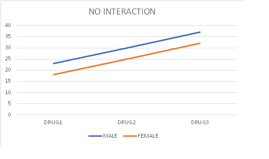
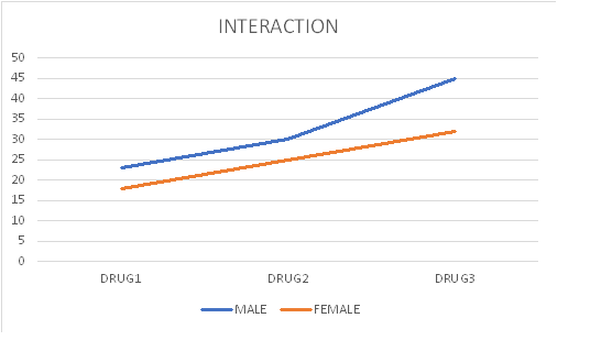
Note the term "Interaction" in the ANOVA summary table of the factorial design What is interaction? The best way to grasp the concept of interaction is to graph it.

INTER1-3


INTER-3-2


ANOVA 2x3 factorial practice example


An experimenter wanted to test the effect of two drugs on the emotionality of male and female teenagers. He randomly selected 15 male and 15 female teenagers and randomly assigned them to 6 groups: Group 1, Group 2, Group 3, Group 4, Group 5, Group 6. five subjects in each group as shown in the following table.


Drug 1
B1

Drug 2,
B2

Drug 3,
B3


Male
A1

A1B1 Group1

Subject 1
Subject 2
Subject 3
Subject 4
Subject 5

A1B2 Group2

Subject 6
Subject 7
Subject 8
Subject 9
Subject 10

A1B3 Group3

Subject 11
Subject 12
Subject 13
Subject 14
Subject 15


Female
A2

A2B1 Group3

Subject 16
Subject 17
Subject 18
Subject 19
Subject 20

A2B2 Group4

Subject 21
Subject 22
Subject 23
Subject 24
Subject 25

A2B3 Group2

Subject 26
Subject 27
Subject 28
Subject 29
Subject 30


The data are presented on the table below. The scores are the values recorded on a device measuring galvanic skin response, a measure of emotionality. Higher values indicate stronger emotion.


B1

B2

B3


A1

A1B1
11
11
13
12
10

A1B2
17
18
17
16
17

A1B3
27
25
24
26
27


A2

A2B1
15
14
14
16
15

A2B2
20
19
18
20
18

A2B3
30
29
29
28
31

.

2x3 FACTORIAL ANOVA SUMMARY TABLE

Source

SS

df

MS

F

p

Between A

67.5

1

67.5

62.31

<.0001

Between B

1088.07

2

544.04

502.19

<.0001

AxB (interaction)

3.8

2

1.9

1.75

0.1952

Within

26

24

1.08


Total

1185.37

29


After we calculate the F, we go to the F table to find the required F value for A, B, and AxB (interaction). Because,( remember?) the F ratio is A over within, B over within, 

AxB over within, we enter the F table with
df of A and df within , which is 1 and 24.
also B and df within, which is 2 and 24
and lastly AxB within., which is 2 and 24. We first choose the F table at 0.05 level of significance.

Factor A: The F at df 1 and 24 is 4.25. In the summary table we see that the F for factor A (rows) is 62.31. This is greater than 4.25, so we conclude that here we have significance at the 0.05 level of significance; we say p<0.05, p less than 0.05. It has been accepted among scientists that at the 0.05 level we are allowed to say that we have significance, that the finding of our experiment is reliable.

Next we look at factor B. We enter the F table with df 2 and 24 and find F=3.50. This is less than the F of our summary table 502.19, therefore we conclude that we have significance at the 0.05 level. We formally express this as follows: p<0.05.

Next we look at AxB. We enter the F table with df 2 and 24 and find F=3.50.. This is greater than the F at the summary table value of 1.75 so we conclude that here we do not have significance. We formally express this as follows: p>0.05.


Step by step calculation of 2x3 ANOVA factorial

The goal of our calculations in ANOVA is to compute the F ratio, The F ratio is MS between over MS within. Mean Square is the mean of the squared deviations (differences).

of each score from the mean. These are very simple calculations involving high school mathematics. Simple as they are, they are very important concepts in data analysis and beyond, that is science in general. You will never need to perform these calculations. There are many free Statistics calculators online. However, for the purpose of developing the concepts of ANOVA here are the steps:

1. Calculate the mean of each group.
2. Subtract each score from the mean.
3. Square each difference
4. Add these squared differences. font red This is the Sum of Squares, the SS on the ANOVA summary table.)
5. calculate the degrees of freedom df (number of scores that went into the calculation of the mean minus 1)
6 Divide the SS by the df. Voila! this the MS.
7. The last step is to calculate the F. Divide MS by the MS of the error term (which is the MS within but may be something else depending on which ANOVA design you have. )


The F ratio, as all ratios, compares two things. For example the ratio 8/4 compares 8 to 4 and finds that 8 is two times greater than 4.


Story 16B — Example 2 of a 2x2 factorial experiment

A pharmacology graduate student

working on his thesis wanted to

find whether a new chemical,

DOP-Y, which has been shown to

elevate dopamine levels in the

brain, may be beneficial to

depressive patients. He was also

interested to see if electroshock

has an effect on these patients

when combined with DOP-Y.

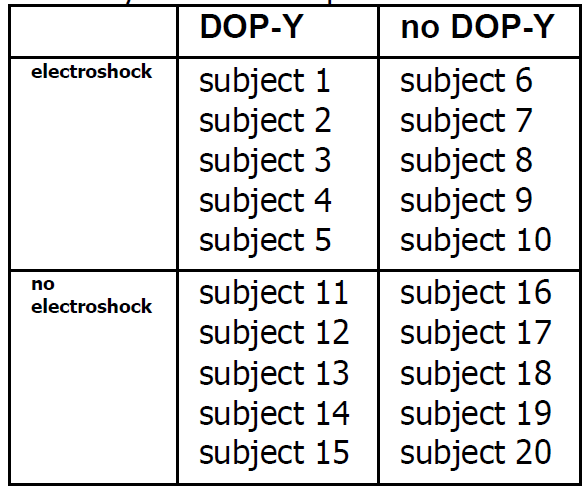
He randomly selected 20

depressive patients, and randomly

assigned them to 4 groups:


electroshock - DOP-Y,

electroshock-no DOP-Y

no-electroshock - DOP-Y,

no-electroshock-no DOP-Y


The layout of the pharmacology experiment


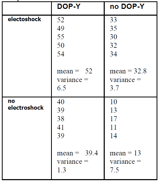
The data he recorded are given in

the next table.

The data of the pharmacology experiment


High numbers indicate improvement.


The data of the pharmacology experiment

THE PHARMACOLOGY EXPERIMENT 

ANOVA SUMMARY TABLE


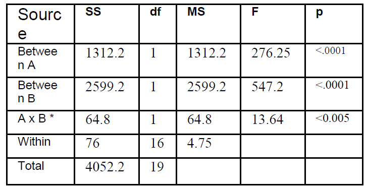
In this table we see that A, B, and

 AxB are significant.


Significance in A means that

electroshock benefited the

depressive patients.


Significance in B means that drug

benefited the depressive patients.


Significance in AxB means that

there was an interaction between electroshock and drug.


Not clear, you say,


You are correct.


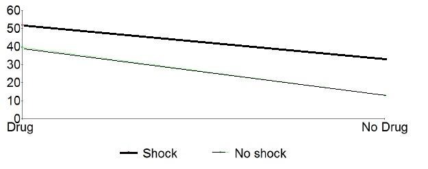
Let us look at the graph of the

interaction.

First, we observe that the two lines,

shock and no shock, are not

parallel. Every time we have an

interaction, the two lines are not

parallel.


Every time we have an interaction,

the two lines are not parallel.


How about getting to understand

interaction at the gut level, not just

with words? you say.


Let’s do it. Look at the graph

above (previous page).


First, we will visualize the graph

without the effects of the drug. In

that graph the two lines would be

parallel.


Now visualize the effect of drug as 

a force pushing the lines up.

Logically we would expect to see

both lines pushed up while

maintaining the distance between

them, i.e., the two lines may move

higher on the graph, but they

should remain parallel. However,

in the present experiment we saw

that the drug has pushed the no

electroshock line

disproportionately higher.

This is the concept of interaction.


Understanding the 2x2 factorial ANOVA summary table


A
Looking at the layout tables above, we see that factor A is gender. Factor B is drug. Our calculations gave a p value <0.05 meaning that factor A, gender, gave a significant difference. In other words, there is a difference in emotionality between male and female

B
Looking at the layout tables above, we see that factor B is Drug. Our calculations gave a p value <0.05, meaning that factor B, drug, gave a significant difference. In other words, there is a difference in emotionality between subjects that received drug 1 as compared to subjects that received drug 2.

AxB
This is the interaction term. Definition of the interaction. What is interaction in factorial designs? Interaction is present if one level of one factor has a disproportionate effect on one level of the other factor.


Story 16 — Examples of 2x2 factorial experiments ANOVA

Example 1 of 2x2 factorial experiment ANOVA


A pharmacology graduate student

working on his thesis wanted to

find whether a new chemical,

srt-X, which has been shown to

block serotonin, may be beneficial

to schizophrenic patients. He was

also interested to see if

electroshock has an effect on

these patients when combined

with srt-X.


He randomly selected 20

schizophrenic patients, and

randomly assigned them to 4

groups:


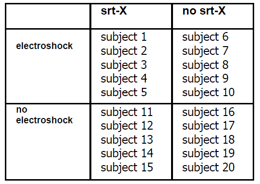
electroshock - srt-X,

electroshock-no srt-X

no electroshock - srt-X,

no electroshock-no srt-X


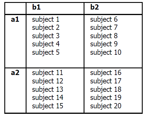
The layout of this experiment is:


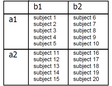
The layout in abstract form is:


Variable A has two levels, a1 and

a2, and variable B has two levels,

b1 and b2.


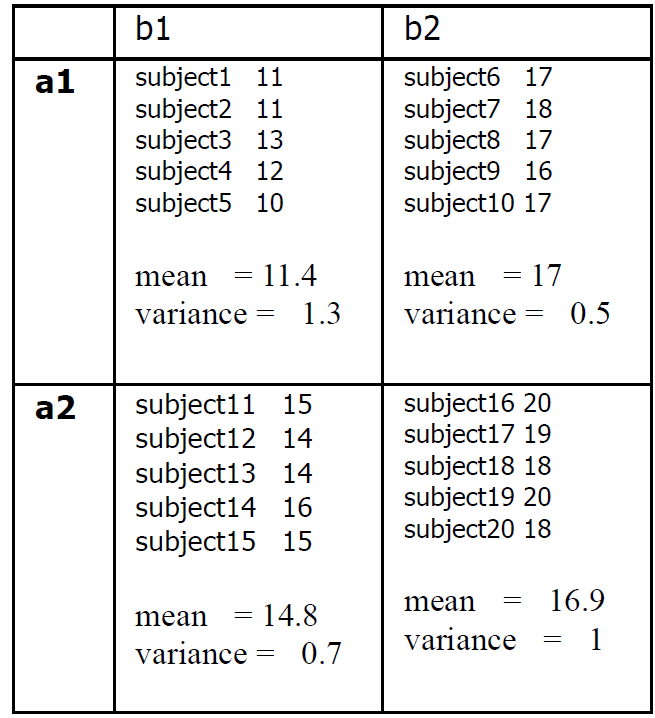
The next table shows the data he

recorded in running the

experiment. The numbers

represent scores on a psychiatric

test measuring intensity of

schizophrenic behavior. The

higher the number the worse the

condition of the patient.


THE SEROTONIN BLOCKER

PLUS SHOCK EXPERIMENT


ANOVA SUMMARY TABLE OF

THE SEROTONIN BLOCKER

PLUS SHOCK EXPERIMENT


* Interaction


I will first discuss the table in terms

of the calculations we did.


First and most important, the

degrees of freedom.


If you tell me the degrees of

freedom in any ANOVA

experiment, but without the use of

formulas (I do also mean resorting

to memory for the recollection of

formulas - ban formulas!), I know

you know what you are talking

about. Calculation of the F is easy,

high school arithmetic.

If you


If you tell me the degrees of

freedom, I know you know how to analyze that data.


Why df for Between A is 1?


Because in order to calculate

variance Between we line up the

means, consider them scores, and

calculate the variance using the

one and only formula for variance

(all the other formulas for variance

that you may see around are

derived from this formula.

Statisticians get their kicks by

producing equivalent formulas, of

considerable complexity and

ornamental value!). Now you and I

know that in order to calculate 

variance, we must first calculate

the mean. Every time we calculate

the mean, we lose 1 degree of

freedom. Because, in the present

example we have 2 scores (never

mind that they are means), we are

left with 1 df. That is 2-1=1.


I do not understand why you say

we have 2 means for A, you ask.


Good question. A has two levels

here, a1 and a2. That is shock and

no shock. You see, when we deal

with variable A, we ignore variable

B. In other words we reduce this

part of the analysis to a one-way,

single-factor ANOVA.


Why df for Between B is 1? you

say.


For the same reasons as in the

previous paragraph, B has two

levels, b1 and b2, drug and no

drug. There are two means

(scores). In order to calculate the

variance of these two scores, we

must first compute the mean. We

therefore lose 1 df. So the df for B

is 2-1=1.


Why df for AxB interaction is 1?


This is easy. Since df for A is 1, and

df for B is also 1, the df for AxB is

1x1=1.

Why is the df for within 16

This is simple, too. We said variance

Within-group SS is computed as the sum

of (n_i - 1)s_i^2 across all groups.

Then MS within = SS within / (N - k),

where k is the number of groups. We have four

groups here. In order to calculate

the variance of each group we

must first calculate a mean. The

consequence of this is that we

lose 1 df for every mean we

calculate. How many scores go

into the calculation of variance for

group 1? Five scores. Therefore

df for the first group is 5-1=4. We

calculate the variance of the

remaining 3 groups in a similar

way. Since we have 4 groups

here, the df for Within is 4x4=16.

he 

Note: Checksum. The sum of df

for A, B, AxB, Within, equals df

Total


SS for A, B, AxB, and Within

equals SS Total.


Remember, we said that in ANOVA

we partition variance.


Discussion of the experiment

with the schizophrenic patients.


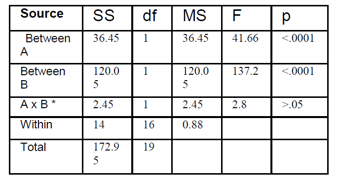
Look at the ANOVA Table again:


ANOVA SUMMARY TABLE OF

THE SEROTONIN BLOCKER

PLUS SHOCK EXPERIMENT


  * Interaction


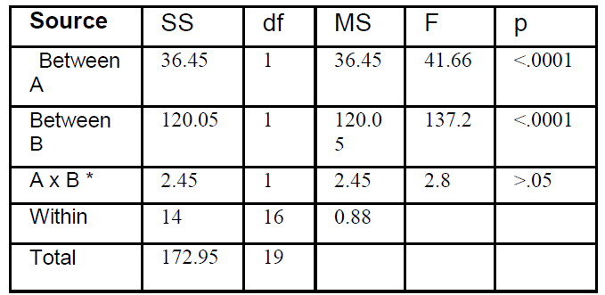
The p value (the probability that

the difference or effect we are

reporting may not be reliable or

significant) for A is less than 1 in

ten thousand (p<.0001|). 


Variable A is electroshock in this

experiment. This means that the

two conditions, electroshock and

no electroshock (condition 1: 

electroshock-drug, electroshock-no drug; condition 2: no-

electroshock-drug, no- electroshock-no drug) produced a result, a significant difference. 

In other words those patients who received electroshock ended up different from those patients that did not receive electroshock. 


The p value (the probability that the difference or effect we are reporting may not be reliable or significant) for B is less than 1 in ten thousand (p<.0001|). 


Variable B is drug in this experiment. This means that the two conditions, drug and no drug (condition 1: drug-electroshock, drug-no electroshock, condition 2: no drug-electroshock, no drug-no electroshock) produced a result, a significant difference. In other words, those patients who received the drug were different from those patients that did not receive the drug. 


The p value of AxB, the interaction 

is p>.05, We read this as follows:

p greater than five per cent. This

means that if we were to say that

there was significant interaction

between electroshock and drug,

we would be running the chance

of reporting an effect that is not

reliable, not significant, meaning

that if we or someone else were to

do the same experiment again,

most likely would not find a

difference as we did

As we said earlier the concept of

interaction is a new one for us,

and we need to understand it our

way, at the gut level, as we are

used to.


We will now consider an experiment in which the interaction is significant.


Story 16 — Analysis of Variance Factorial Designs

Analysis of Variance

Factorial Designs

Two-Way ANOVA


The ANOVA that we discussed so

far is called 'One-way ANOVA' or

'Single-factor ANOVA'.


Now we will consider two-way

ANOVA or two-factor ANOVA.


The concepts we developed so far

also apply to two-way ANOVA.


What do you mean by one-way,

single-factor, two-way, or

two-factor? you say.


Drama

Beam storm


Rutgers College. May 9, 1999, 9:00 in the

morning. Two sections of Statistics 101 are in class: two adjacent classrooms, C120 and

C121. USS Spaceship Enterprise flew over the two classrooms and locked on the bio readings of the students. Then, classroom C120 was bombarded with a X-Z-LOBX beam for 10 milliseconds. The security cameras recorded an almost imperceptible tilt of the head to the left, while the professor of Statistics, without being aware, wrote the same complex formula for MS 5 times. Two nanoseconds after classroom C120 was bathed in the benevolent X-Z-LOBX beam, classroom C121 was bombarded by the same X-Z-LOBX beam for 100 milliseconds. All students raised the index finger of their right hand and stuck it in their left nostril. The professor started reciting the t-table but stopped short in a deluge of laughter from the students.

The duration of the students’ responses was

recorded by the spaceship and instantly

transmitted to Houston where a robot was

waiting to manually enter the data on the

layout of the experiment. The layout of the

experiment was made public, the data not. 

Discussion of data was forbidden by a

unanimous decision of the Congress.


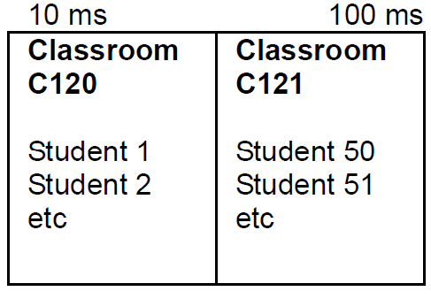
The layout of the USS Enterprise

experiment


This experiment is a one-way

ANOVA design.


Why? Because each student was

bombarded with one beam.

We also say that this design is a

single-factor ANOVA.


Why?


Because each student was

bombarded with a single beam.

Another way of saying this is, that

each score in this experiment is

the result of one beam, one factor,

or one treatment. You may also

 come across the term 

one-way classification.


What we do to the subjects is

called:

independents variable

or treatment


Now it will be easy for us to

understand two-way ANOVA.


An example of a two-way

ANOVA


A psychiatrist wanted to see

whether a combination of wine

and vitamin C may have an effect

on depression.


He randomly selected 10 male

patients, and also 10 female

patients, and randomly assigned

them in two groups: wine group, or

vitamin C group.

.

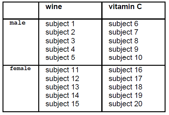
The layout of this experiment is

presented in the next table:


Look at subject 1. This subject is

influenced by two variables. Male

gender, and also wine. The score

of depression that he will give, will

be the result of these two factors.

For this reason, we call this type of

experiment a two-factor

experiment. The same, of course,

holds for all subjects. They are, in

a way, under crossfire. Two

factors hit them.


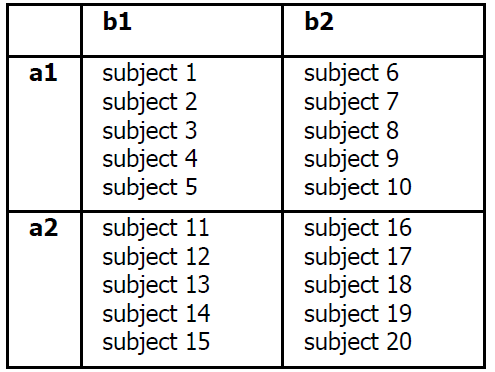
The layout above can also be

given in a more abstract form.


Variable A is gender, variable B is

nutrition. Each variable has two

levels, a1 a2 and b1 b2


We say: We have two variables,

A and B. A is gender, B is nutrition.

Each of these two variables has

two levels. a1, a2, and b1, b2.

Because in this experiment we

use 2 variables with 2 levels each,

we call this experiment 2 x 2

factorial. We read this as follows:


two by two factorial.


The ANOVA summary table for

two-factor experiments is the

following:


ANOVA SUMMARY TABLE

Two-Way, 2x2 Factorial


* Also called interaction


Things are getting complicated, I

hear you say.


I say: You already know everything

in this new ANOVA.


Our approach of understanding

the concepts and not memorizing

formulas has paid out.


Why do we have two Between

terms, A and B? you say.


Because here we have two

variables: gender, and nutrition,

i.e., A and B. We want to know if

gender (being male or female) has

an effect, and also if nutrition (wine

or vitamin C) has an effect.

Remember, the Between term is

the term that senses the effects of

our treatments.


The Within term we also know. It is

the variance of each group

separately. The sum of these

variances.


The Total term we also know. It is

simply the variance of all scores

without regard to what group they

came from.


The interaction term is a Between

term for cells taken diagonally:

mean for a1b1+a2b2 and mean

a1b2+a2b1. Look at the layout to

visualize this.


What is new here is the concept of

the interaction term. We need to

develop this concept, so we get a

gut feeling for it.


When you give two treatments to

subjects, one of the things you

want to see is whether the two

variables interact with each other. 


To begin developing the concept

of interaction, let us consider a

simple experiment:


We give 5 mg of an anti-anxiety

drug, such as diazepam, and find

that this results in an increase in

the time patients sleep. This

increase is 2 hours.


Using different subjects, we find

that 200 ml of wine increase sleep

time by 1 hour.


Now if we give both 5 mg of

valium and 200 ml of wine, is it

sure that we will get 3 hours

increase in sleep time? Perhaps

yes, perhaps no. We know that

drugs may interact and produce

dramatic results, if given together.

You may have heard of cases in

which diazepam taken together

with alcohol caused coma, and

even death, because of

potentiation.


Students find the concept of

interaction difficult. For this reason

I will give an example later.


For the purposes of calculation of

this term in the ANOVA, there is no

problem. The df, as you would

expect, is the df of A x the df for B.


The SS you can calculate by

subtraction. SS total-(SS Between
 

A+SS Between B+SS within).


Alternatively, you can compute the

SS for AxB the same way you

calculated the between term, but

here calculate two means

diagonally, i.e. 

mean for

a1b1+a2b2 

and mean for

a2b1+a1b2. 


Then we proceed with

the calculation of the variance of

these means.


The type of ANOVA design we are

discussing here is called factorial,

because in designing the

experiment we produce all

possible combinations.


In the above example we have:


Male - Wine, Male Vitamin C

Female - Wine, Female Vitamin C


Read this several times, it sounds

like a nursery rhyme. There is a

symmetry in it.


Visualizing the layout of

factorial designs


You will often come across

experiments that use these

designs, and if you go to graduate

school there is good chance you

will use them in your research.


We need to be able to visualize

the designs in order to understand

and evaluate them. A key

part of the task of a scientist is to

be able to critically evaluate the

research of others. Regrettably,

even reputable journals publish

research that is not sound.


We have considered so far a 2x2

design. How do we visualize this?

We see two characters (forget that

it is the number 2 here) separated

by the symbol x which stands for

times.


We have two things, two

variables, we therefore write down

A also B.


A                B


Now we look again at 2x2 and this

time pay attention to what number

we have. Here we have 2.

We therefore write

A

a1 a2


Then we look at the number after

the x. It is also 2 (mind you it does

not have to always be 2, it can be,

4, 10 any number).


We therefore write

B

b1 b2


To sum up:

a1b1 a1b2

a2b1 a2b2


Read this several times, it sounds

like a nursery rhyme. There is a

symmetry in it.


This is how we visualize a 2x2

factorial:


a1b1      a1b2

a2b1      a2b2


Now let us consider this: 2x3 a1b2

a2a2b2

How do we visualize this? We

see two characters (forget that it is

the numbers 2 and 3 here)

separated by the symbol x which

stands for times. We have two

things, two variables, we therefore

write down A and also B.


A           B


Now we look again at 2x3 and this

time pay attention to what

numbers we have. Before x we

have 2. We therefore write:

A

a1 a2


Then we look at the number after

the x. It is 3 (mind you, it does not

have to always be 3, it can be 4,

10, any number).


We therefore write:

B

b1 b2 b3


This is how we visualize a 2x3

factorial:

a1b1      a1b2   a1b3

a2b1      a2b2   a2b3


Now let us consider this: 2x3x5


How do we visualize this? We see

three characters (forget that it is

the numbers 2 and 3 and 5 here)

separated by the symbol x which

stands for times. We have three

things, three variables, we

therefore write down A, B, 

also C.


A     B     C 


Now we look again at 2x3x5 and

this time pay attention to what

numbers we have. Before x we

have 2.

We therefore write

A

a1 a2


Then we look at the number after

the x. It is 3 (mind you, it does not

have to always be 3, it can be, 4,

10, any number).

We therefore write

B

b1 b2 b3


Then we look at the third

number after the x. It is 5 (mind

you it does not have to always be

5, it can be, 6, 28, any number).

We therefore write

C

c1 c2 c3 c4 c5


Story 15 — Analysis of variance One-way ANOVA

Analysis of variance is used by

scientists in order to analyze data

from experiments of literally

unlimited experimental designs. It

is most popular and dominant

statistical test in the biological and

social sciences. The complexity of

these designs ranges from very

simple to frighteningly convoluted.

The formulas are so many that no

statistical book contains all of

them.


As I promised you, we will

navigate through this ocean with

no formulas. We do not need

them. If we understand what we

are doing, if we get the concepts

involved, we do not need

formulas. Do you need a map in

order to work around your

kitchen?


Hurray, here we launch the big

ocean liner, ANOVA! 


What is ANOVA, what do we do in

Analysis of Variance?


We analyze variance.


That is tautologous, you say.


Ok, we partition the variance. That

is pretty much what we do.


Variance I know well, you say.


Analysis of Variance you know

pretty well, I say. 


Yes. Variance we know so well.


wps


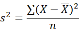
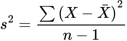
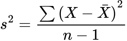
Remember? The sum of squared

deviations of each score from the

mean, and all of this divided by n,

the number of scores that went

into the calculation, i.e., here, the

number of all scores.


Why do you say “here”, you ask.


Good observation. n does not

always represent the number of

scores in an experiment. It is the

number of observations, that is a

safer way to say this. More of that

soon. I was saying that what we do in

ANOVA is analyze the variance in

our data, more specifically, we

partition the variance.


What is the result of this analysis?

Is it a t?


Something like a t. A modified t, I

would say.


You said earlier that it is a modified z. 


t is a modified z

F is a modified t?


You are very observant. Yes. As I

told you earlier, statistics is like a

pyramid. Discoveries are based 

on earlier discoveries.

There is continuity. If you brush

aside the many formulas and

concentrate on concepts, you get

a marvelous view of the edifice of

statistics. Then you are in

command. You can take decisions,

be in a position to critically view

experiments, defend yourself

against criticism that is thrown at

you, and ultimately add this

knowledge to your personal

philosophy.


Drama

Clip his tail


Fisher was determined to clip Gosset ‘s tail

a bit.


That Gosset, he thinks he is smart. He

rides high in the world with his stupid

t-distribution. Big deal! All he did was to

add one puny column on the left of the

normal distribution. The df column. Oh,

yes, ok, ok…He did recalculate the z, big

deal.


Fisher had been scratching his head for

months, engaging in obsessive dialogues

with Gosset, downgrading his achievement

but deep down he knew he was jealous.


I got to come up with something myself.

What if I add another column to the

normal distribution. Another column of

what? Not df again? If not df, what then.

I got to be more original. How about

another line on top of the t table.

He did. The df Between.  

Good Knighthood, Sir Fisher.


The result, the endpoint of

ANOVA, is F. This is in honoring

Fisher who developed ANOVA.

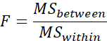
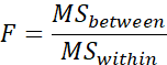
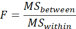
We calculate the F by the so

called F ratio which is:


We read this as follows:


F equals mean square between,

divided by mean square within.


Remember that mean square is

another way of saying variance.

So, you should not be worried with

the F ratio.


What about between and within?

you say.


That is easy. In computing the

variance between we calculate a

variance. We line up the means of

the various groups in our

experiment, we treat them like

scores, and figure out the

variance.


You are kidding, you say. I have

seen terrifying formulas for even

the simplest ANOVA.


You are correct.


Now the second part of your

question. Mean square within.

Easy again. You already know it.

We compute the variance of the

first group, and write it down, then

we compute the variance of the

second group and write it down,

then we do the same for all the

groups in our experiment. The

number of groups can vary from 2

to as many as you wish. In the end

we pool these variances, weighting each by its degrees of freedom.

This gives MS within: sum of (n_i - 1)s_i^2 divided by (N - k).


Amazing! you say. No new

formulas for ANOVA!


You can use ANOVA right away. All

you needed was to get the concepts of variance between and

variance within.


What about partitioning the

variance? you say.


Variance between and variance

within, if added together, give us

the Total variance.


Total variance can be computed if

you calculate the variance of all

the scores of all your groups,

disregarding what group a score

came from. Again, all you need is

the familiar variance formula.


That is unbelievable, you say. I am

confused. Every statistics book

gives ANOVA summary tables.


Yes indeed. That is the

convention, but it is not necessary

in order to compute the F ratio. In

practically every case in which

step by step instructions are given

(without first developing the

concepts) things acquire an aura

of awesome complexity and

difficulty, and, I am afraid, fake

importance.


Because you and I cannot go

against the whole world, let’s take

a quick look at the typical

presentation of ANOVA. Up until

the sixties, journals were including

ANOVA summary tables in the

publications. As I said, this gives a

publication the semblance of

quantitative science, but, alas,

at times only a semblance.


ANOVA SUMMARY TABLE

One-way ANOVA


Source

SS

df

MS

F

p

Between


Within


Total


We know every term on this table.

Within is also called the error term.

The error term is the term which

goes in the denominator of the F

ratio. In more complex designs,

the error term may be other than the

within term.


Review the five formulas that are

needed for virtually all parametric

statistics. Do not simply memorize

them, look into them conceptually


wps


An example of ANOVA


A biologist wanted to see if

quantity of vitamin C in diet may

reduce body weightHe randomly

selected 15 male rats and

randomly assigned them to the

following three groups. Group1 10

mg, Group2 20 mg, and Group3

30 mg. He added this vitamin in

the food of the rats daily for 30

days. On the 30th day he weighed

the rats.


 Here are the data and the

ANOVA table.


GROUP 1 10 mg

GROUP 2 20 mg

GROUP 3 30 mg

200

203

199

190 

204


204

210

214

219 

211

214

220

225

220

229

Mean 1 = 199.20

Mean 2 = 211.60

Mean 3 = 221.6

s = 5.54

s = 5.50

s = 5.68


ANOVA SUMMARY TABLE

One-way ANOVA


Source

SS

df

MS

F

P

Between

1259.2

2

629.6

20.24

≈0.000143

Within

373.2

12

31.10


Total

1632.4

14


The analysis showed that we have

a significant effect. The differences

between the means are

significant, i.e., reliable. The p

value is less than 1 in 10000. This 

means that the probability that the

difference we report is a chance

event (and not the result of our

treatment of giving rats vitamin C)

is less than 1 in 10000.


How did you compute the degrees

of freedom, df, you ask.


You know this if you know the

concepts of Between, Within, and

Total.


We said, in order to compute the

variance between, we line up the

means of all the groups and treat

them as scores, and calculate the

variance. In this balanced design, multiply the sample variance of the group means by the common group size to obtain MS between. How many means we

have here? We have three means.

We really consider them as scores

here. In order to calculate the

variance of three numbers, we

must first calculate the mean. By

calculating the mean, we lose 1

degree of freedom for every mean,

remember? So, our df for the

between term is 3-1=2. 


We calculate variance within as

we said above. We calculate the

mean of the first group and then

the variance of this group. Then

we do the same for the second

group, and then the third group.

We add these 3 variances and this

gives us the variance within. Since

we compute 3 means in the

process of calculating the

variances, we lose 3 degrees of

freedom. How many scores went

into the calculations of variance

within? All the sores, that is 15.

Our degrees of freedom then are

df=15-3=12.


Easy, no formulas needed,

because we understand the

concept of df and also variance

within.

Lastly, we compute the df of Total

as follows:


In order to compute the Total

variance, we said, we take all of

the scores of all the groups 

disregarding what group each

score comes from. In order to

calculate this variance we must

first calculate the mean, therefore

we lose 1 degree of freedom. How

many scores went into the

calculation of the Total variance?

All of the scores, here 15. Our

degrees of freedom for Total then

is 15-1=14.


Note that adding up the df for

Between and Within we find the df

for Total. 


That is what we meant by

partitioning. We said we partition

variance. 


Here we partition the Total

 variance into variance

between and variance within.

Indeed, verify that SS between

plus SS within equals SS Total.

That is,

1259.2 + 373.2 = 1632.4
 

How did we get the p value? you

ask.


I will be very practical here. As

was the case with the t-distribution,

here too, there is a table with the F

values (see Appendix).


These are in a way the recalculated 

1.96, that is the point on the curve

 beyond which 5% of the curve lies.


In the case of the t curve we

entered the table with the degrees

of freedom and found the required

t at the 5% level. In the present

case, we enter the F table with the

degrees of freedom for Between

(in the present experiment df=2)

and the degrees of freedom

for Within (in the present

experiment df=12). We locate the

F on the table. This is the required

F.


Then we compare the obtained F

(the one we calculated, look at he

summary table) to the required F.

As in the case of the t-test, if our

obtained F is greater than the

required F, we have significance.

We then say p<0.05.


I understand how we calculate df

without formulas, however I do not

see why we need it.


I see why you are confused. As I

said this is what happens every

time we try to teach in a

mechanistic, compulsive, step by

step way. The general practice of

working with formulas blindly, and

using the ANOVA summary table,

often prevents the student from

seeing what is going on.

As I said at the beginning, the

ANOVA summary table is not

needed. What you need to do is

simply calculate the variance, and

compare the variances, that is the

F ratio. df is simply the n in the

variance formula. 


df is simply the n in the variance

formula


 I understand variance Between,

variance Within, and df.

However, I do not see why the F

ratio can detect significance, you

say.


A very important question, if

indeed, we are sincere when we

say we want to understand the

concepts and the logic of statistics.

Drama

Master of the waves


It is a beautiful, cool, calm day in

Puerto Rico. You are sitting in a San

Juan small café, nested on the rocks

overlooking the magnificent Atlantic

ocean. You are happy, sipping your

coffee, Bacardi on the side, and slowly

nibbling on a sinfully sweet piece of PR

cake. It is quiet, the only thing you

hear is the rhythmic sound of waves

gently breaking on the foundations of

the cafe. Suddenly you hear voices; it

sounds like people are arguing. Soon

their voices become loud enough, you

can clearly hear what they are saying.


You don’t believe me? Look again.

See? caused that wave.


There is much laughter.


Buddy, you are nuts, that’s what I

say. The only waves you cause is in

your brain. You go and see a shrink!


The argument grows in intensity and

the guy with the claims to

supernatural powers, keeps throwing

small stones into the sea. You decide

to join the noisy group and get the

argument straight.


Guys, I have the answer to your

argument. I will show you who is

right. For now, let the sea rest and

calm down, just in case this guy has

disturbed it. Come sit and have a cup

of coffee.


Ten minutes later, you take the lot to the edge of the rocks.


First, we will measure the heights of the next 40 waves and record these data, you say.


When forty waves have been recorded, you

turn to the guy with the supernatural claims

and say:


Ok, this is your show now.


The guy, his confidence somewhat deflated,

picks up a stone and hurls it into the sea. All

eyes are fixed on the base of the rock, waiting for the next wave. The wave comes and is recorded.


The moment of truth, you say.


The height of the wave is read out loud. It is

not taller than any of the 40 waves previously recorded. The miracle worker receives a truckload of cosmetic epithets and soon the café slips back into the beatific serenity. Sleep hovers over your eyelids. You dream of conquistadors and 

fierce Carib Indians, of rituals and dances that humans created in an attempt to understand their world. 


Cute story, but I still do not

understand why the F ratio can

indeed measure that we have

significance, you say.


The forty waves provided us with

what I call the “endogenous”

variance, baseline, the variation in

the heights of the waves that is

present when no obvious cause

can be seen. The wave after the

action of the ambitious miracle

worker was the presumed effect of

his manipulation (in statistics we

call this treatment). Comparing the

baseline with the claimed effect of

his manipulation can give us

support, or lack thereof, for a

connection between what he did

and the result we observed.


If the result which he claims that

he caused by his manipulation is

bigger than the natural,

(endogenous or spontaneous

variance), then we may say that

he caused the effect by his

manipulation.

A brief parenthesis at this point to make

sure we understand what we mean by

saying ratio. Alas, mechanistic methods

of teaching arithmetic without

development of concepts, often prevent

the pupil from understanding that in

division, what we do is compare two

numbers: the numerator to the

denominator. If you have 20 dollars, and

I have 5 dollars, in dividing 20 by 5, I

compare 20 to 5. You have 4 times

more money than I have.


Our treatment causes variance

between to increase? you say.


Yes, let’s see it in an example.


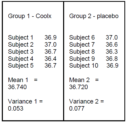
A pharmacologist is testing a new

drug (tentatively named Coolx)

that is suspected to lower body

temperature. He randomly

selects 10 male college students

and randomly assigns them to

two groups. Group 1 receives

Coolx, Group 2 receives a

placebo (an inert substance that

has no effect on physiology).


Here is the layout of the

experiment.


Group 1 Coolx

Group 2 Placebo

Subject 1

Subject 2

Subject 3

Subject 4

Subject 5

Subject 6

Subject 7

Subject 9

Subject 9

Subject 10


Before the experiment proper, the

pharmacologist records the

temperature of the subjects, in

order to have the baseline

temperature, the temperature that

is present without any

manipulation on the part of 

the experimenter.


Here is the baseline temperature

(Celsius)


We will now calculate variance

between.


Remember, in order to calculate

variance between we line up the

means and treat them as scores.

We then proceed and calculate the

variance of these scores.


Here we have two means

36.740   36.720

The variance of these two scores

is 0.0002. This is variance between.


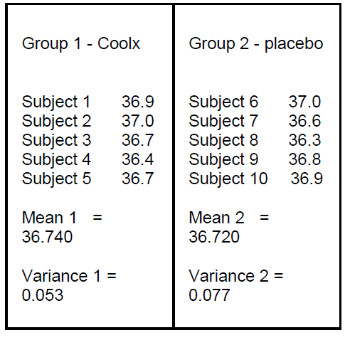
The next table shows temperature

after the administration of drug

Coolx to Group 1


Note that the mean in Group 1

decreased. It was 36.740 before

giving the drug, it is 35.94 now.

Also note that the variance of this

group did not change.


Now the big moment has arrived.

Has the variance between

changed? If yes, we will be

convinced that variance between 

is sensitive to our manipulation,

i.e., that it senses the effect of the

drug.


As usual, in order to calculate

variance between, we line up the

means and treat them as scores.

We then calculate the variance of

these scores.


The means here are:


35.94 36.720


The variance is 0.3042.

This is variance between.


Let’s compare this to variance

between before our manipulation

of giving the drug:


We saw above that variance was

0.0002 .


Voila! After giving the drug, that is

after our treatment, variance

between changed. Variance within

did not change.


Conclusion: The F ratio is

sensitive to our treatment. It does

so, because variance Between

changes because of our

manipulation, while variance

Within does not change.


Why? you say.


Remember that variance

measures the distance of scores

from the mean. The mean can

increase or decrease but the

distance of scores from the mean

does not change. The scores

move up or down with the mean.


Story 14 — An example of the t-test


An example of the t-test


A sports physiologist suspected

that bouillon cubes may improve

the performance of runners. She

got this idea when she read a

1996 experiment of mine in the

Journal of Physiology and

Behavior. She randomly selected

12 U of I male undergraduates

and randomly assigned them to

either group 1 who were given a

cup of soup with a bouillon cube,

or group 2 who were given a cup

of chamomile.


She subsequently asked the

students to run a 100 meter

course and recorded the time they

took to reach the finish line.


Here is the layout of the

experiment.


GROUP 1 BOUILLON


SUBJECT 1

SUBJECT 2

SUBJECT 3

SUBJECT 4

SUBJECT 5

SUBJECT 6

GROUP 2 NO BOUILLON


SUBJECT 7

SUBJECT 8

SUBJECT 9

SUBJECT 10

SUBJECT 11

SUBJECT 12


Note that a subject belongs to only

one group, so the groups are

independent. If subject 1 is John,

and he belongs to the first group,

he does not participate in the

second group.


When the data were collected,

she analyzed them by using the

t-test. We say she ran a t-test.


The data and analysis are

presented in the next table:


Bouillon 

No Bouillon


34 

35 

39 

30 

39 

40 

48

 47

 45

 47

 46

 45

Mean 

36.17 

46.33

Variance 

14.97 

1.47

df 

 10


 6.14


 0.000109


What do you mean by df? you

say. You look unhappy too.


In order to develop the concept of

degrees of freedom, df, we will run

tought experiment (thought

experiment) as Einstein used to

say. The benefit will be that you

will not need to memorize any of

the many formulas for degrees of

freedom. Ever.


Drama

Mean Prophet


I take a sheet of paper from my printer

and cut it into four equal pieces. I take a

pencil and write the number 3 on the first

piece, I write number 4 on the second

piece, number 8 on the third piece, and

lastly number 5 on the fourth piece of

paper. I place all four pieces of paper in a

shoe box and put the cover on it so that

the pieces of paper cannot be seen. On

another sheet of paper I keep a record of

these four numbers. Then I add them up

3+4+8+5=20. Then I calculate the

average or mean.


20 divided by 4 equals 5. The mean is 5.

I destroy this piece of paper.


I take another sheet of paper and I write

on it the following:

Mean=5 n=4


I stick this paper on the shoe box for

anyone to see.


I ask Jerry, the English major who is

sitting in the lounge, to come into the

room. I explain to him that there are 4

pieces of paper in the box, each having a

number on it. The mean of those numbers

is 5. That is all he is told.


I begin by asking Jerry:

Jerry, close your eyes, stick your

hand in the shoe box and pick one

of the four pieces of paper.

Jerry does that. Before he draws

his hand out of the box I ask him

to guess the number he has picked.

Jerry giggles.


I am not a magician, he says.


Open your eyes and read out the

number.


Eight, he says.


I lay the piece of paper with the

number 8 down on the table so

that it can be seen at glance at

anytime.

Now Jerry, stick your hand again in

the shoebox and pick another piece

of paper. Jerry does so. Before he

draws his hand out of the box, I

ask him to guess the number he

has picked.


Again, Jerry giggles and mumbles:

No way!

Open your eyes and read the

number out loud.


Five, he says.


I lay the piece of paper on the

table next the first one that Jerry

picked, the one that has the

number 8 on it. It can easily be

seen. There are two pieces of

papers on the table now with the

numbers, 8 and 5.


I repeat the procedure for the third time.


Jerry, can you guess what the number that you drew?

He smiles faintly and simply shrugs his

shoulders.


Open your eyes and read the number out loud.


Four, he says.


Again, I lay the piece of paper with the number 4 on the table, next to the other two. There are three numbers on the table now:

8 and 5 and 4.


We are ready to repeat the procedure, I say. Close your eyes and stick …


Before I can finish my sentence, Jerry says:


Number 3.


Great! Jerry knows simple

arithmetic. He added up the

numbers he had already drawn.


8+5+4=17. There is only one

number which, if added to 17, will

give 20. That is the number 3.

There is only one number that

divided by 4 will give us a mean of

5. That number is 20.


What am I to get out of this story?

you say.


Without knowing the mean and the

n (how many numbers) you could

not guess any of the numbers.

They were free to vary. Several

arrays of four numbers could give

us a sum of 20. For example

11+1+2+6=20, or 5+ 6+8+1=20.

Because I calculated the mean

and showed it to you, and I also

told you how many numbers there

are in the box, one of the numbers

is not free to vary.


In statistical language we say: We

lose one degree of freedom every

ime we calculate a mean.


We lose one degree of freedom for

every mean that we calculate. 

mean we calculate.

Remember this.


The degrees of freedom in this

case is 3, that is

4-1=3.


Formally we write it as follows:

df=3.


In another situation that we have

two groups of 10 subjects each, 20

total, and we calculate two means

the degrees of freedom are 18. That

is, we subtract 1 for each mean

we calculate. This is simple to

remember. I am confident that you

understand this concept at the gut

level, not just repeating my words

like a parrot.


As I promised you, we will push

aside almost all the formulas that

otherwise you would have to

memorize.


It is logical, isn’t it. If you know the

concept and you know what you

are doing, you do not need a

formula to tell you what to do step

by step.


Back to our discussion of the

t-test.


Definition: t obtained.


That is the result of solving for t. In

other words when you run a t-test

you find a t value. A third way of

saying this is: the result of

analyzing your data using the t

formula.


Definition: t required.


The required t is the value

contained in the t-table which is

found in the end of every statistics

book, including the one you are

reading now (see Appendix).


Remember, the t-table lists the

modified 1.96 that Gosset

published. It lists the recalculated

values for 1.96 depending on

degrees of freedom.


To find the required t, you first

calculate the degrees of freedom.

You are an expert in calculating

degrees of freedom (df). No

formulas needed, not for us who

learn statistics by acting in soap

operas.


In the present example of the

t-test (page 114) we have two

groups of 6 subjects each, total of

12 subjects. Since in computing

the t we need to first compute the

mean of each group, two means,

we lose 2 degrees of freedom.

How many scores go into the

calculation of the t? All of the

scores. That is,12 scores, minus 2

equals 10. Therefore, df=10.

Now we go to the t table in

Appendix and run our finger

down the left column which is 

labeled df. We stop at 10. Then we

draw out finger horizontally until

we reach the column that is

labeled 2.5% or 0.025 for a two-tailed 0.05 test. We copy the

value we find at the tip of our

finger. This is the required t.


We compare this with the obtained

t, i.e., the one that we calculated. If

the obtained t is larger than the

required t, we have significance.

We say that our finding (the

difference between the two

means) is reliable or significant.

This means that we trust that, if

we run the same experiment

again, we will find a difference

again.


We formally write this as follows:


The difference between the means

of the two groups is significant

(p<0.5).


By that we mean that the finding

we are reporting is reliable, but

there is still a chance that it may 

not be “real”. That chance is less

than five per cent. Scientists

around the world have agreed to

accept findings for which the

probability of being chance events

and not “real“ is less than five

percent. You understand correctly,

there is no absolute certainty in

experimental natural science.

Findings are taken to be “true” on

a probability basis. You see that

boring, compulsive statistics

borders on philosophy if

approached from the correct

angle.


One last remark. It is really

unwarranted to speak of truth in

dealing with phenomena in the

empirical, material world. We can

only speak of truth in the formal,

logical and mathematical

sciences. 


Two plus three equals five. This

 is true. Two plus three is

six, is false. It makes no sense to

say that the statement: “Valium at

doses of 2, 5, 10, and 20 mg

reduces anxiety” is true. It is

simply reliable and there is a

probability attached to it, no matter

how small, that it may not be so.


Story 13 — The t-test


William Sealy Gosset

(June 13, 1876–October 16, 1937)

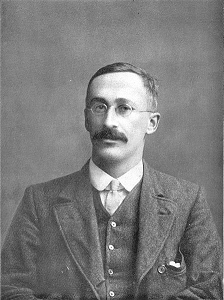
Wikipedia Aug, 2014 PD


William Sealy Gosset published

the t-test under the pen name

Student. We refer to the

distribution of this test as the

t-distribution. The t-test is a test of

inference, i.e., it allows us to infer

on the basis of our data, whether

the difference between two means

is reliable or, as we say, significant.


In what follows, we will first try to

develop the concepts needed for

understanding the logic and the

operations involved in the t-test.


We will talk about this and that and

the other. Be patient. Then we will

go over an example of the t-test.

Developing the concepts in the

t-test


As is the case with all parametric

tests that we will cover in this

book, the t-test analysis is based

on variance.


In experiments in which we have

two groups we analyze our data by

using the t-test. There are two

types of t-tests. The t-test for

independent samples (groups),

and the other for dependent or

paired samples. Here we will

consider independent samples.


What are independent samples?

you say.


Ok. We will make a small

parenthesis in order to develop the

concept of independence.


Drama

Apple-pie IQ

A psychologist has a sneaky suspicion that

the type of apple pie has an effect on

intelligence. She randomly selected 20

students and randomly assigned them to

two groups. Group 1, golden delicious

apple pie, Group 2, red delicious apple pie.

John Gluck was assigned in Group 1, and

his friend Paul Crust was assigned to

Group 2. The psychologist proceeded with

giving these subjects a pound of apple pie

to eat. Subsequently she tested their

intelligence. Each subject was allowed to

see their intelligence score. There were 20

intelligence scores, one for each subject.

These groups are independent as you see.

She analyzed her data by using a t-test for

independent groups in order to see if there

was a significant difference in intelligence

in the two groups.


Note: An unexpected event occurred during the running of the experiment. One of the subjects in Group 2 did not show up on time so the experiment was delayed for a few minutes. John Gluck, who, as you remember, was in Group 1, offered to participate in Group 2, in addition to his participation in Group 1. The experimenter did not allow this. Had she allowed John Gluck to be a subject in both groups, she would have violated the rule of independence, and she would not have been able to analyze her data by using the t-test for independent samples.


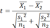
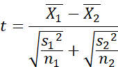
The formula for the t-test is:
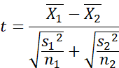


We read this as follows:


T equals mean 1 minus mean 2

divided by the square root of the

variance of group 1 and group 2

divided by the number of scores

that went into the calculation of the

variance.


Faithful to our goal we must

understand the concepts in the

t-test.


First look at the numerator. 

Mean 1 minus mean 2, that is the

difference of the two means.


Next look at the denominator.

The square root of the variance 

is the standard deviation. 

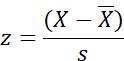
This looks like the z formula that

 we considered above. Here it is again: 
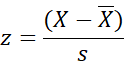


Yes, you say, but the numerator of

the z formula is score minus the

mean. The numerator of the t-test

formula is mean 1 minus mean 2.

Where is the mean? They are not

the same, you say.


They are the same, I say. Mean 1

minus mean 2 is the difference

between the two means. Gosset

treats this difference as a score.


Yes, you say, but then where is

the mean in the t-formula?


The mean is there!  I say.


It is there but you do not see it. It

is 0. The mean is zero.


The mean is zero!


Let the drums thunder at this

point. Let the bugles sound in the

four corners of the world!


The normal (t-) distribution with 0

in the middle. In other words, a

curve with a mean of 0.


 A most important point in the history of

statistics. 


Let us call this curve the

curve of no difference.


I do not understand the t formula

at the gut level, you say.


Watch the ritual dance with the

t-formula.


Drama

An archetypal ceremony II


I have a difference between

the two means. I hold this

difference up, wave it in the

air, I baptize it score. Then I

wear my glasses and stick my

nose on the t curve, running

up and down the line with

standard deviations on it, and

mumble: where does this

score fall? Where does this

score fall?


I then use the z formula -

oops, the t-formula - and

find where exactly our score -

oops, our difference - falls.


This is an archetypal ceremony.

Remember? Amazing, isn’t it? The

t-formula is actually the z formula!

I promised you that you do not

need the mind-boggling array of

fear inspiring formulas. Hang on.


Here is more of the story of the t

distribution. The motive in

Gosset’s mind was to modify the

normal curve so that it could safely

be used for small samples. He

decided to make it difficult for

researchers to find significance

(i.e., to decide whether the

difference between our two means

is reliable) when the samp

les are

small. The curve he created is a

normal curve with some intriguing

qualities. The noses, or tails of the

curve lift up as the sample size

decreases. The tails of the curve

lift up. You can see that in the graph that follows.


The shorter (lower) curve

corresponds to the smaller sample.
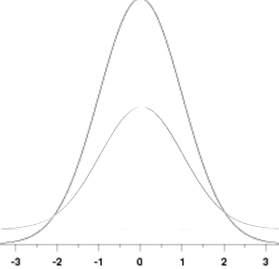


 T-CURVES


What an ingenious idea! 

Some of you, few, very few,

already see what this means. It

means that it becomes more

difficult for you to find significance

because the percentage of the

curve increases in the tails so that

the magic standard deviation of

1.96 becomes larger, which in turn

makes it difficult for you to find

significance, that is to have a

“real” effect, a “true” finding so that

you can publish your experiment.


Let’s finish this story of the t-test,

a statistical test that is used so

frequently in labs across the world

daily.


So far, we have said that we have

two groups, therefore two means,

two standard deviations. We are

interested in deciding whether the

difference between the two means

is reliable, i.e., that it is not a

chance event, that it is, in a sense,

real. We find the t, which is

actually a z, that is, it tells us

where on the curve this difference

falls.


Ok, you say. So, we find the t

which is like z, then what?


If our sample is large the t

distribution is identical to the

normal distribution. In the normal

distribution, we have seen that z of

1.96 is an important mark.

Between -1.96 and +1.96 95% of

the curve falls. A score (here a

difference) that falls within these

two marking points, has a

probability of 95% to occur by

chance in a known situation in

which there is no difference, that is

in a situation in which the two 

samples were drawn from the

same population. That is what our

curve of no difference graphs.


If our sample is small? you ask.


While in the normal distribution

1.96 always marks the 95% of the

curve, in the t distribution it is so

only if the sample size is very

large. With smaller samples, 1.96

is replaced by a larger critical t that changes nonlinearly with

degrees of freedom. The smaller the

sample, the farther the critical t is above

1.96.

Remember, again, Gosset’ s goal

was to make it difficult for

researchers to find significance

with small samples. He calculated

these new values of 1.96.


Drama

Mercy Mr. Gosset


Mr. Gosset, good morning. This is

Samir calling from India. I ran an

experiment with 20 subjects. How

much should I increase 1.96?


Half asleep, Gosset takes out his notes

and read the value to Samir.


The new value for z 1.96, the t, is

2.101.

Good night Mr. Samir.


Two hours later the phone rings again.


Good evening, Mr. Gosset. I am

Michel Duzed, calling from Montreal

Canada. Please give me the value of z

for an experiment with 72 subjects.

Gosset looks at his notes and says:


It is 1.994

Goodnight.


Going back to sleep is difficult for Mr. Gosset. One hour later the phone

rings again, this time from Japan.


Good day Mr. Gosset. Please give me

the new z for an experiment with 402

subjects.


1.966, Gosset says, and he hangs up.

I got to do something about this, he

says, aside from pulling the phone

from the plug. I got to do something…

I will never be able to sleep.


He did. He published his notes

with the recalculated z of 1.96.

Have you seen this in any

statistics book? All of my students

say no, actually a lot of my

colleagues say no, too. I will

disclose the secret. It is the

famous t-table found at the end of

every statistics book, including the

one you are reading now (see

Appendix). Promise to keep our secret between us.


Climax in the drama.


Samir of India wrote down the t

value: 

2.101


With hands trembling he picked up

the sheet with the data analysis of

his thesis to find the result of the

t-test. He read it out aloud:


t=2.24

I made it! I made it!


he chants as he dances around in

his room. Samir will get his

Masters. The difference between

the two means of his experiment is

reliable.


He will report his finding as

significant. In his thesis he will

write:


This difference is significant

(p<0.05).


What does this notation mean?


It means that the chance that his

finding is not reliable, i.e., that it is a

chance event, is less than 5 per

cent.Scientists have agreed to accept

findings as being reliable if the p

value is less than 0.05.


Scientists have agreed to accept

findings as being reliable, 

if the p value is less than 0.05.


Remember this!


Back in Canada Michel Duzed, holding the

note with the t value that Mr. Gosset just

gave her (it was 1.994, remember?),

compares it with the result of the t-test

value that she got by analyzing the data of

her experiment, which was t=1.982.


Alas! The t she computed by using the t

formula is smaller than the t Mr. Gosset

gave her.


Her eyes open wide, her face get gloomy,

and she collapses on an armchair. Michel

will not get her Doctorate. Her finding is

not significant. She will not write her

dissertation. If she were to write it, she

would report it as follows.


This finding is not significant (p>0.05).

P greater than 0.05.


This means that her difference could have

been a chance event more than 5 times in

a hundred.


Michel quits graduate school, she marries

her sweetheart and moves out of Quebec

to a job as a business consultant.


What happened to the Japanese

guy?


Standard deviation 1.96

Percent of curve 95%

Standard deviation 2.56

Percent of curve 99%


The curve of no difference, as we

said, has zero in the middle, that is

the mean is zero. 


What does this curve graph?

 Remember the curve in the case

 of the woolen caps for the farmers 

of the State of Wisconsin? 


That curve was a curve

that we would be getting if we

were allowed to collect many

samples, figure out the mean of

each, and graph these means. In

effect this curve was empty. 


But remember we knew

something about it. We knew the

estimate of the standard deviation

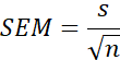
(standard error of the mean). We

calculated it from the standard

deviation of the one and only

sample mean we had.

In our present case, the t-curve is

a similar curve. It would be

graphing differences between two

means, if were we allowed to run

our experiment of two groups

many times, each time having two

means, calculating the mean of

each group and then calculating

the difference of the two means.


Because we have the standard

deviation of this curve, we can

consider our difference as a score

and engage in the ritual dance of

where my score falls. What point

on the standard deviation line

does this score (difference) lie.

We used the z formula to tell us

where on the curve our difference

lies. We said above that the

t-formula is actually a z formula, a

modified one, to take into account

the sample size. Let’s look at them

again.
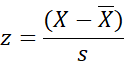


z equals score minus the mean

divided by the standard deviation.


t equals score (mean 1 minus

mean 2 gives us the difference

which we consider to be a score)

divided by the standard deviation

(the standard deviation of both

groups; remember that the square

root of variance is the standard

deviation).


You see then that the t is a z.


Why is the variance of each group

divided by the number of subjects

in the group?


Remember, Gosset’s goal was to

make it difficult to researchers to

find significance if their sample 

size was small.


Understanding the logic of the

t-curve, the curve of no

difference.


Drama

Me minus me equals 1


Professor Lilly Prydum, a statistician,

decided to run a simple experiment to test

a model for guessing if two means came

from one specific group, or they came

from two different groups.


Quite convoluted, you say.


She invited Memy Tallibum, Ph.D. in

Education, to be part of the experiment

and try to guess if the difference of two

means came from the same group, or not.

The subjects were 30 students from

Trenton College. They were asked to take

a test of 120 questions on Chinese

geography, mythology, and culture. The

scoring of the test was done by a

computer, and the recording of the data

was done in such a way that the subjects

remained anonymous. The experiment

lasted 35 days. Subjects were asked not

to read about China during this time

period. They were also asked not to chat

amongst themselves and not to compare

notes. 


Day 1 of the experiment. Time 9:00 in the

morning. The test is given. Time allotted 1

hour. 10:00 a.m. the testing period is

over. Students are asked to take a 30

minute break. During that time the exam

papers are graded, and the score is

recorded next to each subject. Dr.

Tallibum gets a copy of the results and

studies them with care.


At 10:30 the students are called back in

again, and are given the same test, the

one they took 30 minutes earlier. At

11:30 the testing session is over. The

subjects are thanked, and asked to be

back the next day. “Please be back here

at 9:00 in the morning sharp. And

remember, no reading on China”.


The students leave, their exam papers are

graded, and the score of each student is

recorded. Each subject now has two

scores. The score from session 1 and the

score from session 2. Dr. Tallibum gets a

copy and scrutinizes it. As expected the

difference between the first session and

the second is very small, and for most

students it is zero.


The next day all students are present, Dr.

Tallibum is present, and the experiment

proceeds as planned.


Session 1, the students are given the

same test they took the previous day. Session

2, the students are given the same test.

Scores are recorded and are handed to Dr.

Tallibum who watches like a hawk. At the

end of the second day Dr. Tallibum is not

surprised to see that, once again, the

difference between the first and the

second session is very small, close to zero.

Students are reminded that the

experiment will last 35 days, and asked to

“come back tomorrow “.


On day 16 of the experiment Dr. Tallibum

is surprised to see that the difference

between the first and the second session

is substantial. Students did not score as

well in the second session. The

explanation came in the evening as she

was watching the news. Pop star Mickey

Wiggletuchs had died. Students must have

heard about this during the break between

the two sessions and were emotionally

disturbed. That influenced their

performance in the second session.


On day 33 Dr. Tallibum was shocked to

see that the difference between session 1

and session 2 was so great. Scores in the

second session were so low! Again the

explanation came in the evening news.

The stock market had crashed. Apparently

the students heard of this disaster during

the break between the two sessions. Most

likely parents called and told their

children that there would be no money to

pay the college fees.


Day 34, the day before the last day

of the experiment, rolls smoothly.

At the end of the second session,

Dr. Tallibum is asked to leave the

exam room. 


Students are given the same

instructions as usual. They are told

to be present as usual, for the last

day of the experiment.


Dr. Tallibum is left in the dark, she

does not know what the students

were told.


Day 35, the last day of the experiment.


Session 1. Students are taking the test

as in the past and Dr. Tallibum is

present, as in the past. During the

break the exam papers are graded and

scores handed to Dr. Tallibum.


At this point, there is a dramatic

change in the procedure. Dr. Tallibum

is asked to leave the exam room. She

is led to the elevator and taken to the

biology laboratories on the top floor,

where there are no windows. She is

asked not to leave this lab, not to

make any phone calls, and wait there

for an hour. To make sure, she is

guarded by the graduate students of

the biology lab.


At 11:30 the second session of the

experiment is over. The students are

told that the experiment came to an

end, that there was no need for them

to come back again, and were given a

brief talk as to the purpose of the

experiment.


The papers were graded, the scores

were recorded and Professor Lilly

Prydum, the experimenter, took the

elevator to the Biology Lab and

handed the results to Dr. Tallibum.


Dr. Tallibum, she said. In the second

session we prevented you from seeing

who were the subjects. As you realize

we may have used the same subjects,

the students from Trenton College, or

we may have used another group. We

could have used workers from the

Physical Plant of the College, students

from Trenton High, or senior citizens

from the local senior citizens club.

Your task is to guess whether the

group that took the test during today’s

second session of the experiment were

the Trenton College students that you

watched for 35 days, or another,

different group.


Dr. Tallibum looked at the data sheet. It

contained the difference between session

1 and session 2 for 35 days. The difference

score of day 35 was the score in question.


Instinctively, her eyes ran up and down

the list of differences. She was trying to

find if the score of day 35 has occurred in

the past 34 days. Not only that. If it has

occurred, how often has it occurred. If she

finds that it has occurred many times, she

will conclude that the students in the

second session of today were the same

students, that is the Trenton College

students.


If the difference score of today is not on

the list, if it has never occurred in the last

34 days, then the wisest guess would be

that in the second session of today it was

not the Trenton College students that took

the test.


It will be more difficult to guess if the

difference of day 35 has occurred a few

times, very few times. That's where Dr.

Tallibum will resort to her knowledge of

statistics. Guess what. She will draw

Goddess Normal Curve and pray. Let’s

listen to her reasoning out loud:


Dr. Tallibum’s soliloquy


The solution to my problem must be in the

normal curve, as always. What do I have

here. I have a difference between two

means but I do not know if the two means

came from the same group, or from two

different groups. I want to guess wisely. I

will start by placing 0 in the middle of the

normal curve. This is the curve of no

difference. I assume that this curve

graphs differences between means that

come from a known case, a case in which

all means come from the same group, the

same people. If the difference that I am

not sure about is 0 or close to 0, I can

safely conclude that this difference comes

from the same group of people, i.e., that in

both sessions of day 35 it was the Trenton

College students that took the test. If the

difference in question is large …ay, there's

the rub. Whether it safer to say same or

not say, and suffer the slings and arrows

of rough ridicule, or to shut up and by

going against my promise to participate,

my participation end. But behold, there is

light. I can compute the standard

deviation of this no-difference curve and

reason. I can engage in the archetypal

dance.


Behold Dr. Tallibum dancing around the

biology lab to the amazement of the bio

graduate students.


I have a difference between the two

means. I hold this difference up, wave it

in the air, I baptize it score. Then I wear

my glasses and stick my nose on the

normal curve, running up and down the

line with standard deviations on it, and

mumble: where does this score fall?

Where does this score fall?


I then use the z formula and find where

exactly my score - oops, our difference -

falls. If it falls within -1.96 and +1.96 then this score occurs frequently, 95% of the time, in this case of known no difference. If this score, difference, falls beyond 1.96 then it is a rare occurrence.

In this case the wisest guess is that it

does not come from the same group, that

is, in the second session it was not the

Trenton students but another different

group of people.


I hear a question. Speak up.

Can she find out what was this

new group, you say.

Yes, the Oracle of Delphi should

be able to tell you that.


Drama

The long jump


The prototypic experimenter is standing in

the middle of the normal curve holding his

score or difference in his hand. He is

focusing on 1.96 and is about to jump

beyond it. If he succeeds in jumping over

1.96, he gets a medallion (his degree

perhaps); if he does not succeed, he lands

on his behind, and gets a kick on the

same.


Talking seriously now. All statistical tests

are based on the same logic we developed

above. So, I advise you to read my

theatrical masterpieces carefully if you

want to get the concepts, and be able to

reason in statistics, and solve the

problems with only 5 formulas.


What are these 5 formulas?


The five formulas we need to know:
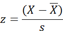


 currently editing the formulas


Story 12 — Normal distribution Use number 4 - reliability of the difference between two means

Normal distribution 

 Use number 4


To make statements

regarding the reliability of

the difference between two means


A psychologist at the University of

California published a study in

which she claimed that college

students who prefer Polish

sausage react faster as compared

to college students who eat plain

hotdogs. She measured the time it

takes to respond when a stimulus,

a buzzer, is presented.


Here is a summary of the data:


Reaction Time ms


Polish

Sausage

Hotdog

Mean 

210

215

Standard

deviation

20

25


The difference between the two

means is 5 milliseconds. The

Polish sausage group responds in

less time, that is this group is

faster. However, a question pops

up: Is this difference reliable?

Which means, will we find this

difference, if we run the

experiment again, or this

difference was perhaps found by

chance.


We can use the normal distribution

to solve this problem. However, it

is the almost universal practice in

many sciences to use the t-test,

the so-called Student's t-test. The

t-test was created by William

Sealy Gosset.


Story 11 — Normal distribution Use number 3 - reliability of a single mean


Normal distribution

 Use number 3


To make stat

regarding the reliability of a

single mean


Drama

A Cap for Wisconsin Farmers


Mike got his degree in Psychology from

UW Madison. Given the large number of

psychology graduates and also his doubts

regarding his suitability for psychology

practice, he found a job as a consultant

with the State of Wisconsin. Psychologists,

you should know, learn a lot of statistics.

Around the middle of last November, his

boss walked into his office and said:


Mike, I have a job for you. The governor

has decided to give a present to all

farmers in the State of Wisconsin because

they are very angry with the new taxes.

The gift will be a woolen cap. We want to

know the size of the cap. If we can find

the average head size of Wisconsin

farmers, we can give the order to a factory

in Milwaukee to make the caps. They are

woolen so they naturally stretch. If we

know the average head size we will be ok.

Since we only have one month to

complete this project, I expect you to

report to me with a plan and budget

tomorrow. 


Early the next morning Mike walked into

his boss’s office and handed him the

proposal. Three hundred personnel to

cover the entire state, to locate every

farmer, in one weak. Fifty 4x4 Jeeps to

safely travel to even the remotest towns.

One small aircraft to land in the northern

towns in case of snow. Three hundred

laptops. Ten German Shepherds to smell

the bears up and around Wausau. Budget.

$30,000.00.


His boss looked at Mike for 20 seconds

speechless. Then, in a completely

unemotional voice, he said:


Mike, in the State of Wisconsin we are

very careful with our money. No way. Find

a less expensive way by tomorrow.


Mike began to fear for his job. All day in

his office, all night in his home, he

scratched his head, drank a lot of coffee,

and prayed to Goddess Normal Curve.


I am not allowed to measure all farmer

heads. That is too expensive. I can,

perhaps, still find a way to use the normal

curve. If I can come up with a mean that

has a strong probability to be close to the

real mean… If I take measures of the

heads of many farmers and compute the

mean…. Can I be sure that this is close to

real mean? If not, I will lose my job. So,

what if I go out a second time and repeat

the data collection, just to make sure that

this mean was not a mean that I got by

chance but it was a mean close to the real

mean. Ah, that might be it! I go out

several times and each time I compute the

mean. In the end I graph these means (as

though they were scores).


Then I use the normal curve to reason

in some way. How? Let me see… The

normal curve would be graphing

means. So, the mean would be the

mean of the means. Can I play the

game of Nick? He was making

probability statements, predictions,

regarding the occurrence of scores,

using the standard deviation of the

scores. Ah! I can use the standard

deviation of the means. Then I can

reason, like Nick, that a mean close to

the mean of means, that is between

standard deviation -2 and +2 would

have a high probability of occurrence.

That’s it!


He prepares the budget, and early in

the morning he busts into his boss’s

office.


It will cost us $10,000, he says.

Good idea, but too expensive.

Tomorrow is the last day, boss says,

and with the palm of his hand he

points at the door.


Three in the morning, Mike is on his knees

in front of Goddess Normal Curve, buried

in statistics books and statistics journals,

and notes from his stat class. Suddenly he

comes across an article in a journal which

claims that you can calculate an estimate

of the standard deviation of the normal

curve that would be graphing means.


…that would be graphing means... Would

be…, he repeats this several times.


Would be, because this curve has only one

mean. Let me say it in another way. You

go out and you collect data from a large

sample. You can calculate an estimate of

the standard deviation of the curve that

would be graphing the means of samples

that you would be getting if you were

allowed to collect several samples.


Weird…, Mike mumbles. What good is it?

I want to be able to collect one sample,

calculate the mean, and tell my boss that

we can trust this mean as being close to

the real head size of Wisconsin farmers,

that it is reliable. What good is computing

an estimate of the standard deviation of a

curve and not know much else about this

curve…


The traffic noise picks up, it is six o’clock

in the morning. Another look at the

Goddess, and a supplication for

inspiration.


All I know is what Nick did, Mike says. He

placed the mean of his data on the normal

curve mean (middle). Unfortunately, I do

not have the mean of the means, since I

am allowed to take only one mean. Let me

place the letters TM in the middle of the

normal curve, TM for True Mean. TM will

remain forever unknown. Pretty spooky.

But I can place the standard deviation of

this “I-would-be-getting” curve, an

estimate of the standard deviation, to be

exact.


Ok, then what.


Weird things happen to people under

stress and in despair. Some people hear

voices, others are visited by angels,

others write poetry…


Got it! he suddenly exclaims, raises the

normal curve over his head, and dances a

cannibal dance around his desk.


Eight in the morning he rushes into his

Boss’s office.


One day, one sample, one mean, one

thousand dollars!  he yelps.


His boss pretends he is not listening.


I will go out, one day, collect many head

size scores, calculate this mean. Next, I

will compute an estimate of the standard

deviation of this curve that you did not

allow me to get the data for. I will then

run down two standard deviations from

the middle of the curve (-2 to +2).


Mike pauses to get some feedback from

his boss. Stone silence.


Grant me this, Mike continues in a loud

voice. This curve would be graphing

means, right? My one mean is one of

these means, right?


That is absolutely correct, and also

tautologous, boss says, and looks at Mike

with contempt. 


What is the chance that this mean

would be one of the 95 percent of

the means? Mike asks.


It’s highly probable, almost certain

boss replies.


Then the problem boils down to the

size of the standard deviation of

this curve, i.e., the estimate that we

will compute. If the standard

deviation is large, then we would

run the risk of producing caps that

are ridiculously large or small for

the heads of Wisconsin farmers. If

the standard deviation is small, our

mean would almost certainly be

close to the true mean, and we are

in business.


Mike carried out this project

successfully without any problems,

except that he was chased by a
playful bear at Wausau up north.


The formula for the calculation of

the estimate of the standard

deviation of the curve that we

would be getting if we were

allowed to get many samples, but

are allowed only to take one

sample, and so have only one

mean, is:


We read this as follows: standard

error of the mean equals the

standard deviation (of the data

from our one sample), divided by

the square root of the number of

data that go into the calculation,

i.e., the n. Yes, you guess right, the

official name for the estimate of

the standard deviation of the curve

that would be graphing means is

called standard error of the mean.


Story 10 — Normal distribution, use number 2 Making statements of probability, betting

Drama

Money in a Texas hat


After taking my course, Nick, an

entrepreneurial mind, decided to go

into business. He went south to

Houston Texas, and planned a

betting business without any

substantial investment. Just an

antique Texas Instruments

calculator. For two months he stood

at a corner in downtown Houston

asking every man that appeared

around the corner:


Excuse me, sir, would you mind if I

measure how tall you are? I am

running my thesis and need data.


He carefully recorded the data. At

the end of the two months he had

measured the heights of 4000 men.

Now he punched his data into the

calculator and computed the mean

and the standard deviation.

The mean was 170 cm, that is 1

meter and 70 centimeters. The

standard deviation was 10.


The next morning, he puts on his

brightest face, and stands at the same

corner in downtown Houston. Time to

make money.


Excuse me sir, I bet $1000.00 that the

first man that will appear around the

corner will be between 1 meter 50

centimeters, and 1 meter 90

centimeters tall.


Not all passersby pay attention to him

but a few do.


Oh Yeah? How do you know, buddy?

You think you are smart, ah? Here is

$1000. Show me yours.


Tom puts down his $1000. Here he

comes, first man appears around the

corner. He agrees to be measured. His

height is 170. Nick wins. Nick will

make several thousand dollars on his

first day. He loses a few times but

95% of the time he wins.

Let’s see his reasoning.


He followed my example of

Basita’s story. He placed the mean

of the heights,170 cm, (the one

that he computed from his data)

on the middle of the normal curve.

Now he reasoned that since the

standard deviation of his data was

10, at standard deviation -1 score

160 exists, at standard deviation

-2 score 150 exists, and at

standard deviation -3 score 140

exists.


Similarly, on the right side of the

curve, score 180 is at standard

deviation +1, score 190 is at

standard deviation +2, and score

200 is at standard deviation +3.


One more example:


Mean 20

Standard deviation 3


What standard deviation score 26

lies at?


Answer: Score 26 lies at standard

deviation +2


At standard deviation +1 we have

score 23, i.e., 20+3


At standard deviation +2 we have

score 26, i.e., 20+3+3


At standard deviation +3 we have

score 29, i.e., 20+3+3+3

At standard deviation -1 we have

score 17, i.e., 20-3


At standard deviation -2 we have

score 14, i.e., 20-3-3


At standard deviation -3 we have

score 11, i.e., 20-3-3-3