Factorial ANOVA

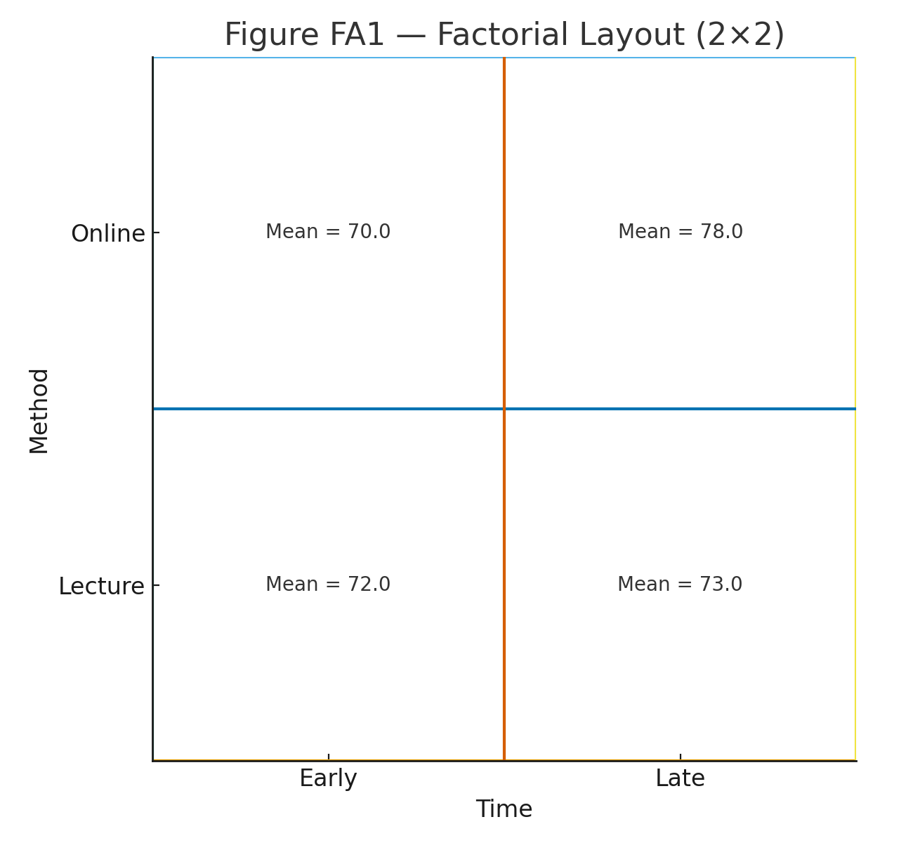
factorial layout
factorial means interaction
factorial interaction

Goal. Test the effects of Method (Lecture vs. Online) and Time (Early vs. Late) on exam scores, and whether there is an interaction between Method and Time.

Design & Experiment

  • Factor A (Method): Lecture vs. Online
  • Factor B (Time): Early vs. Late
  • Balanced design: \(n=5\) per cell ⇒ total \(N=20\).

Students are randomly assigned to one of four cells (Method × Time). After a short module, all students take the same 100-point exam.

Figure 1: 2 × 2 layout (Method × Time).


Data

Scores by cell (five students per cell):

MethodTimeScoresCell Mean
LectureEarly686870727270.0
LectureLate767678808078.0
OnlineEarly707072747472.0
OnlineLate717173757573.0

Within each cell the sample variance is 4 (SD = 2), so the within-cell sum of squares is \((n-1)s^2 = 4\times4 = 16\) per cell.

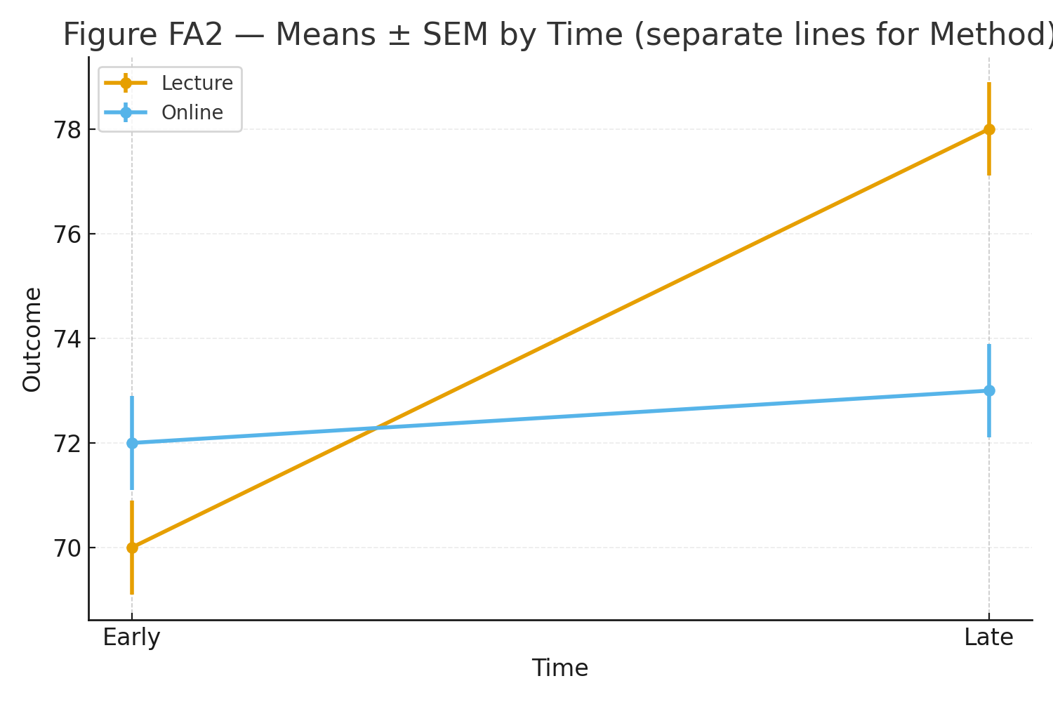
Figure 2: Means with SEM by Time, separate lines for Method.

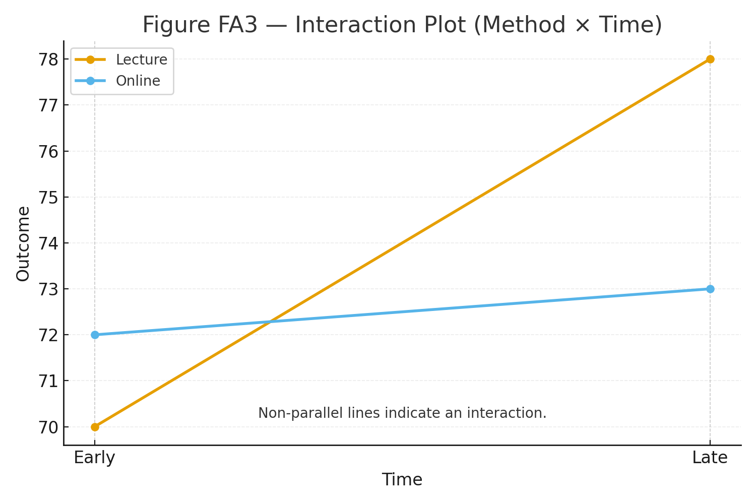
Figure 3: Interaction plot (Lecture rises sharply; Online nearly flat).


Step 1 — Marginal Means and Grand Mean

Cell means: \[ \bar X_{\text{Lecture,Early}}=70,\; \bar X_{\text{Lecture,Late}}=78,\; \bar X_{\text{Online,Early}}=72,\; \bar X_{\text{Online,Late}}=73. \] Marginal means: \[ \bar X_{\text{Lecture}}=\frac{70+78}{2}=74,\quad \bar X_{\text{Online}}=\frac{72+73}{2}=72.5; \qquad \bar X_{\text{Early}}=\frac{70+72}{2}=71,\quad \bar X_{\text{Late}}=\frac{78+73}{2}=75.5. \] Grand mean: \[ \bar X=\frac{70+78+72+73}{4}=73.25. \]


Step 2 — Sums of Squares (Between)

Balanced design formulas (with \(n\) per cell, \(a=b=2\)):

  • \(SS_A = nb \sum_a(\bar X_{a\cdot}-\bar X)^2\), here \(nb=10\).
  • \(SS_B = na \sum_b(\bar X_{\cdot b}-\bar X)^2\), here \(na=10\).
  • \(SS_{AB} = n \sum_{a,b}\big(\bar X_{ab}-\bar X_{a\cdot}-\bar X_{\cdot b}+\bar X\big)^2\), here \(n=5\).

Compute each term:

Factor A (Method): \[ \begin{aligned} SS_A &= 10\Big[(74-73.25)^2 + (72.5-73.25)^2\Big]\\ &= 10\big[0.75^2 + (-0.75)^2\big] = 10(0.5625+0.5625)=\mathbf{11.25}. \end{aligned} \]

Factor B (Time): \[ \begin{aligned} SS_B &= 10\Big[(71-73.25)^2 + (75.5-73.25)^2\Big]\\ &= 10\big[(-2.25)^2 + (2.25)^2\big] = 10(5.0625+5.0625)=\mathbf{101.25}. \end{aligned} \]

Interaction \(A\times B\): For each cell compute \(d_{ab}=\bar X_{ab}-\bar X_{a\cdot}-\bar X_{\cdot b}+\bar X\). Here each \(d_{ab}=\pm1.75\) so \(d_{ab}^2=3.0625\) and there are four cells: \[ SS_{AB}=5\times(4\times3.0625)=\mathbf{61.25}. \]


Step 3 — Within-Group (Error) and Total SS

Within each cell, \((n-1)s^2=16\). With 4 cells: \[ SS_{\text{within}}=\mathbf{64.00}. \]

Total: \[ SS_{\text{total}}=SS_A+SS_B+SS_{AB}+SS_{\text{within}} =11.25+101.25+61.25+64.00=\mathbf{238.75}. \]


Step 4 — Degrees of Freedom & Mean Squares

\[ \begin{aligned} &df_A=a-1=1,\quad df_B=b-1=1,\quad df_{AB}=(a-1)(b-1)=1,\\ &df_{\text{within}}=N-ab=20-4=\mathbf{16},\quad df_{\text{total}}=N-1=19. \end{aligned} \] \[ MS_A=\frac{11.25}{1}=11.25,\quad MS_B=\frac{101.25}{1}=101.25,\quad MS_{AB}=\frac{61.25}{1}=61.25,\quad MS_{\text{within}}=\frac{64.00}{16}=\mathbf{4.00}. \]


Step 5 — F Tests & p-values

\[ F_A=\frac{MS_A}{MS_{\text{within}}}=\frac{11.25}{4}= \mathbf{2.8125},\qquad F_B=\frac{MS_B}{MS_{\text{within}}}=\frac{101.25}{4}= \mathbf{25.3125},\qquad F_{AB}=\frac{MS_{AB}}{MS_{\text{within}}}=\frac{61.25}{4}= \mathbf{15.3125}. \] With \(df_1=1\), \(df_2=16\): \[ p_A \approx 0.11\;(\text{n.s.}),\quad p_B < 0.001,\quad p_{AB} \approx 0.001. \]


ANOVA Summary Table

SourceSSdfMSFp
Method (A)11.25111.252.8125≈ 0.11
Time (B)101.251101.2525.3125< 0.001
A × B61.25161.2515.3125≈ 0.001
Within (Error)64.00164.00
Total238.7519

Interpretation

Main effect of Time (B) is significant: Late > Early on average. Main effect of Method (A) is not significant at conventional levels. The interaction (A × B) is significant: Lecture improves markedly from Early→Late, while Online changes little—non-parallel lines in the interaction plot.

Figure 4: Interaction plot highlighting non-parallel lines.

Assumptions (checklist)

  • Independence of observations within and across cells.
  • Approximately normal scores within each cell.
  • Homogeneity of variances across cells (here, each cell variance ≈ 4).

Practice self-test quiz

In the space below, please find practice problems and self-test quizzes. For full access, please signup free.
One-Way ANOVA

anova boxplot
anova means sem
anova partition variance
anova f distribution

Goal. Test whether three teaching methods lead to different average exam scores.

Design & Experiment

Twenty-four students are randomly assigned to one of three methods (n = 8 per group):

  • Group A: Active discussion
  • Group B: Structured lecture
  • Group C: Self-study

After a 2-week module, everyone takes the same 100-point exam.


Data

Group AGroup BGroup C
727865
688270
758066
707768
697967
738169
718364
747671

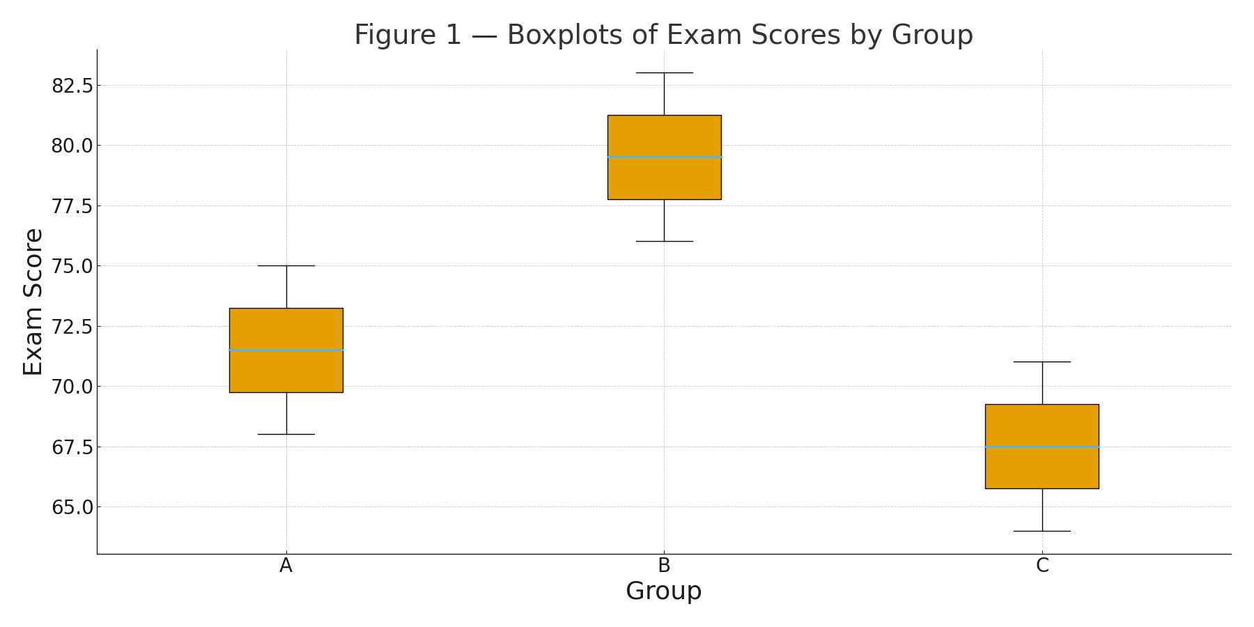
Figure 1: Boxplots of scores by group.

Group sizes: \(n_A=n_B=n_C=8\). Total \(N=24\).


Step 1 — Sums & Means

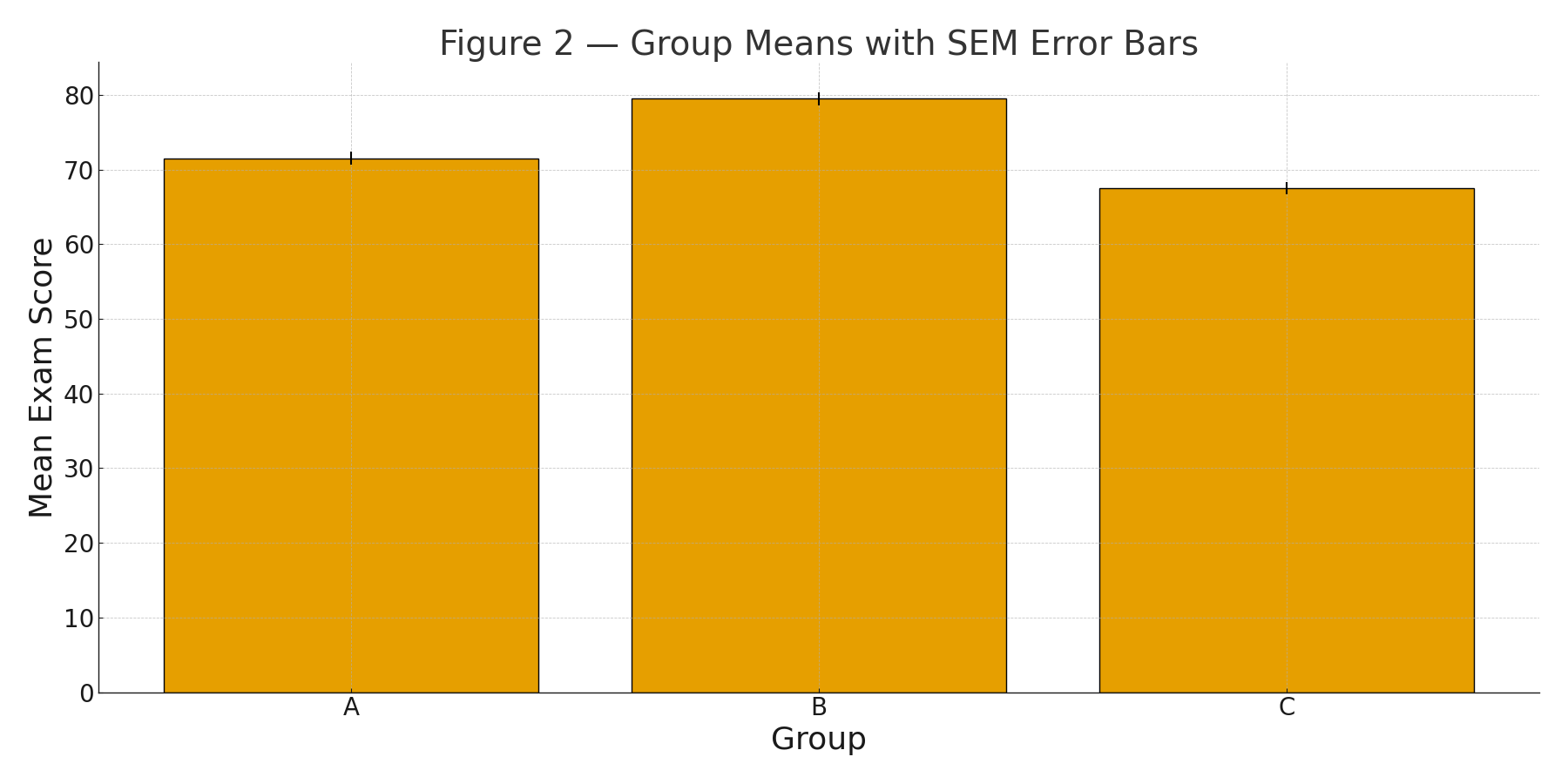
\(\displaystyle \begin{aligned} \text{Sums:}&\quad \sum A=572,\;\; \sum B=636,\;\; \sum C=540.\\[4pt] \text{Means:}&\quad \bar A=\tfrac{572}{8}=71.5,\;\; \bar B=\tfrac{636}{8}=79.5,\;\; \bar C=\tfrac{540}{8}=67.5.\\[4pt] \text{Grand mean:}&\quad \bar X=\tfrac{572+636+540}{24}=72.8333\ldots \end{aligned} \)


Step 2 — Within-Group Variability (sample variances)

For each group, compute \( s_g^2=\dfrac{\sum(x-\bar x_g)^2}{n_g-1} \).

  • \(s_A^2 = 6.0\)
  • \(s_B^2 = 6.0\)
  • \(s_C^2 = 6.0\)

Corresponding sums of squares within each group: \(\displaystyle SS_A=\sum(x-\bar A)^2=42,\; SS_B=42,\; SS_C=42\Rightarrow SS_{\text{within}}=42+42+42=126.0. \)

Figure 2: Group means with SEM error bars.


Step 3 — Between-Groups Variability

\(\displaystyle SS_{\text{between}}=\sum_{g} n_g(\bar x_g-\bar X)^2 =8(71.5-72.8333)^2+8(79.5-72.8333)^2+8(67.5-72.8333)^2 =597.3333\ldots \)

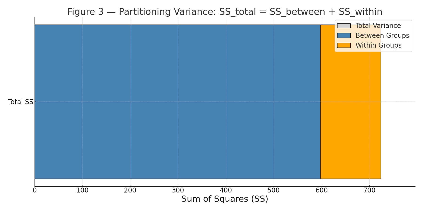
Total sum of squares: \(\displaystyle SS_{\text{total}}=\sum (x-\bar X)^2 = SS_{\text{between}}+SS_{\text{within}} =597.3333\ldots+126.0=723.3333\ldots \)

Figure 3: Partitioning variance (\(SS_{\text{total}}=SS_{\text{between}}+SS_{\text{within}}\)).


Degrees of Freedom & Mean Squares

\(\displaystyle df_{\text{between}}=k-1=3-1=2,\qquad df_{\text{within}}=N-k=24-3=21,\qquad df_{\text{total}}=N-1=23. \)

\(\displaystyle MS_{\text{between}}=\frac{SS_{\text{between}}}{df_{\text{between}}} =\frac{597.3333}{2}=298.6667,\qquad MS_{\text{within}}=\frac{SS_{\text{within}}}{df_{\text{within}}} =\frac{126.0}{21}=6.0. \)


Test Statistic & p-value

\(\displaystyle F=\frac{MS_{\text{between}}}{MS_{\text{within}}} =\frac{298.6667}{6.0}=49.7778. \)

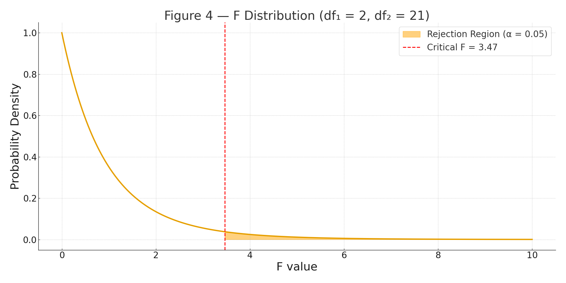
With \(df_1=2\), \(df_2=21\), the (right-tail) p-value is \(p\approx 1.07\times10^{-8}\) (i.e., \(p<0.00000002\)).

Figure 4: F distribution curve with right-tail decision region.


ANOVA Summary Table

SourceSSdfMSFp
Between groups597.33332298.666749.7778< 0.00000002
Within (error)126.0000216.0000
Total723.333323

Conclusion

There is a statistically significant difference among the three methods’ mean scores (\(F(2,21)=49.78,\; p\ll .001\)). A post-hoc comparison (e.g., Tukey HSD) would identify which pairs differ.

Assumptions (checklist)

  • Independent observations (via random assignment).
  • Approximately normal scores within each group.
  • Homogeneity of variance (here, each group variance \(\approx 6\)).

Practice self-test quiz

In the space below, please find practice problems and self-test quizzes. For full access, please signup free.

Table of Contents


Add new comment

Plain text

  • No HTML tags allowed.
  • Lines and paragraphs break automatically.

Story 6 — The Goddess Normal Curve

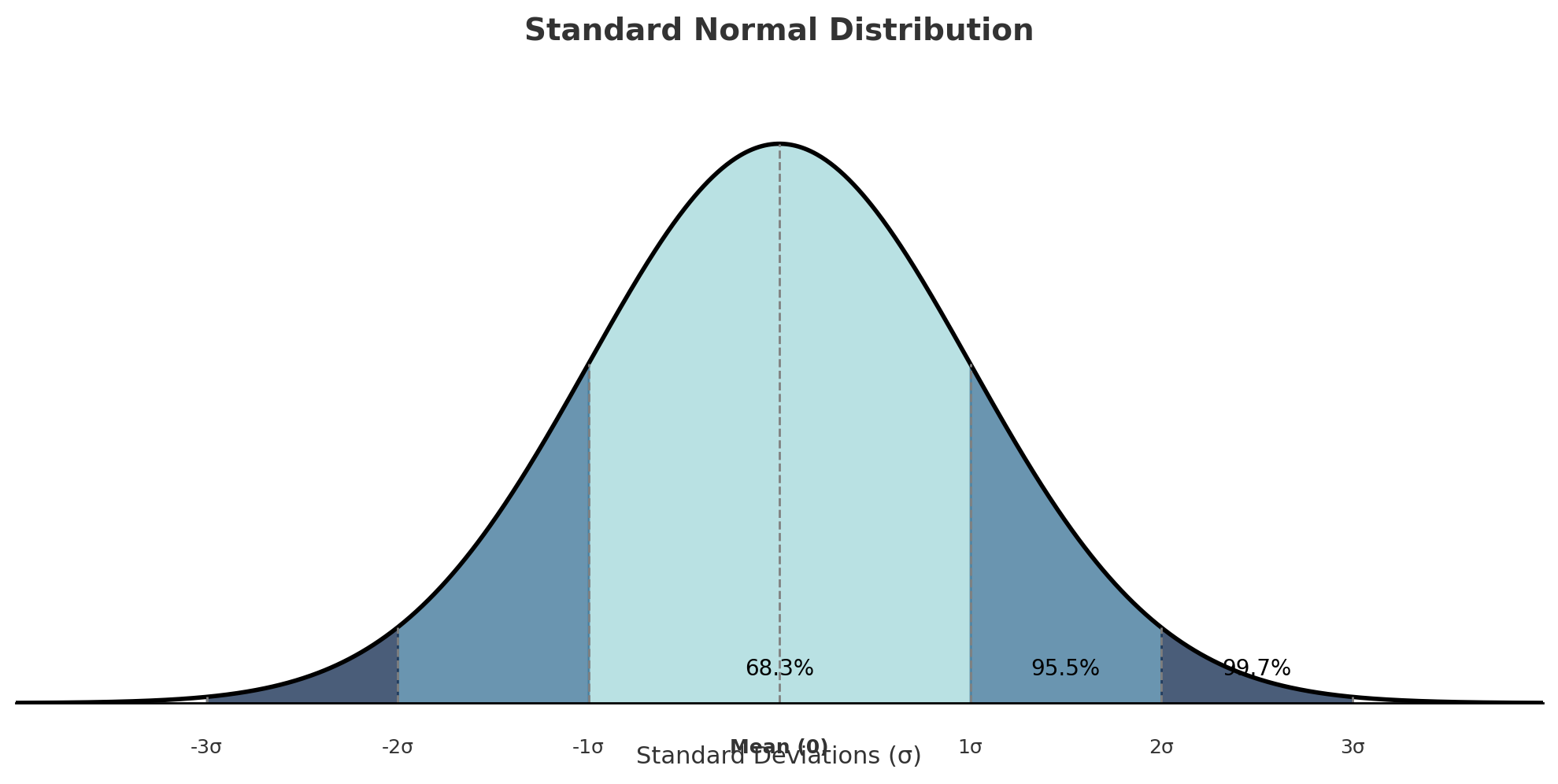
The standard normal distribution

Drama: You Should Bow and Pray

You should bow and pray.
This is Goddess Normal Curve — the mother of all.
Elegant, serene, and, most important, endowed with hidden powers that can guide and reward those who seek her wisdom.

In our long journey across the barren land of Statistics, when confusion and despair arise, we will call upon her for help and inspiration.

Let me put it differently:
Every line of reasoning in this book unfolds beneath her gaze.
Every problem we solve, every doubt we wrestle with, we do so while staring at this goddess, scratching our heads in search of understanding.

Do not be discouraged by the graph you see.
Remember — fifth graders can understand this.


The Shape of Perfection

Take a good look.

She resembles a Texas hat — wide, smooth, perfectly balanced.
Her form is symmetrical.
If you took a pair of scissors and cut her down the middle, the two halves would match exactly — mirror images of one another.

Perfect, isn’t she?

And like all perfection, she does not exist in the material world.
What we see in data — those rough approximations and noisy curves — are mere reflections. The true Normal Curve exists only in our minds.
She is an idea, a concept of balance and harmony.

Mathematicians, moved by this ideal, have captured her form in an equation — the most famous in all of statistics.
(See Appendix.)


The Sacred Geometry

Now, look closely at her base — the horizontal axis.
At the very center lies 0. A vertical line over 0 splits the curve into two equal parts.
To the right of 0, you see two vertical lines; to the left, two more.

These vertical lines mark distances from the center — the measure of how far things stray from the mean.

And thus, balance is born:
for every deviation to the right, there is an equal deviation to the left.

This is the language of the goddess — symmetry, simplicity, perfection.
All of statistics unfolds from this quiet curve, this silent teacher.

Practice self-test quiz

In the space below, please find practice problems and self-test quizzes. For full access, please signup free.

Story 5 — My Zero Is Not Zero

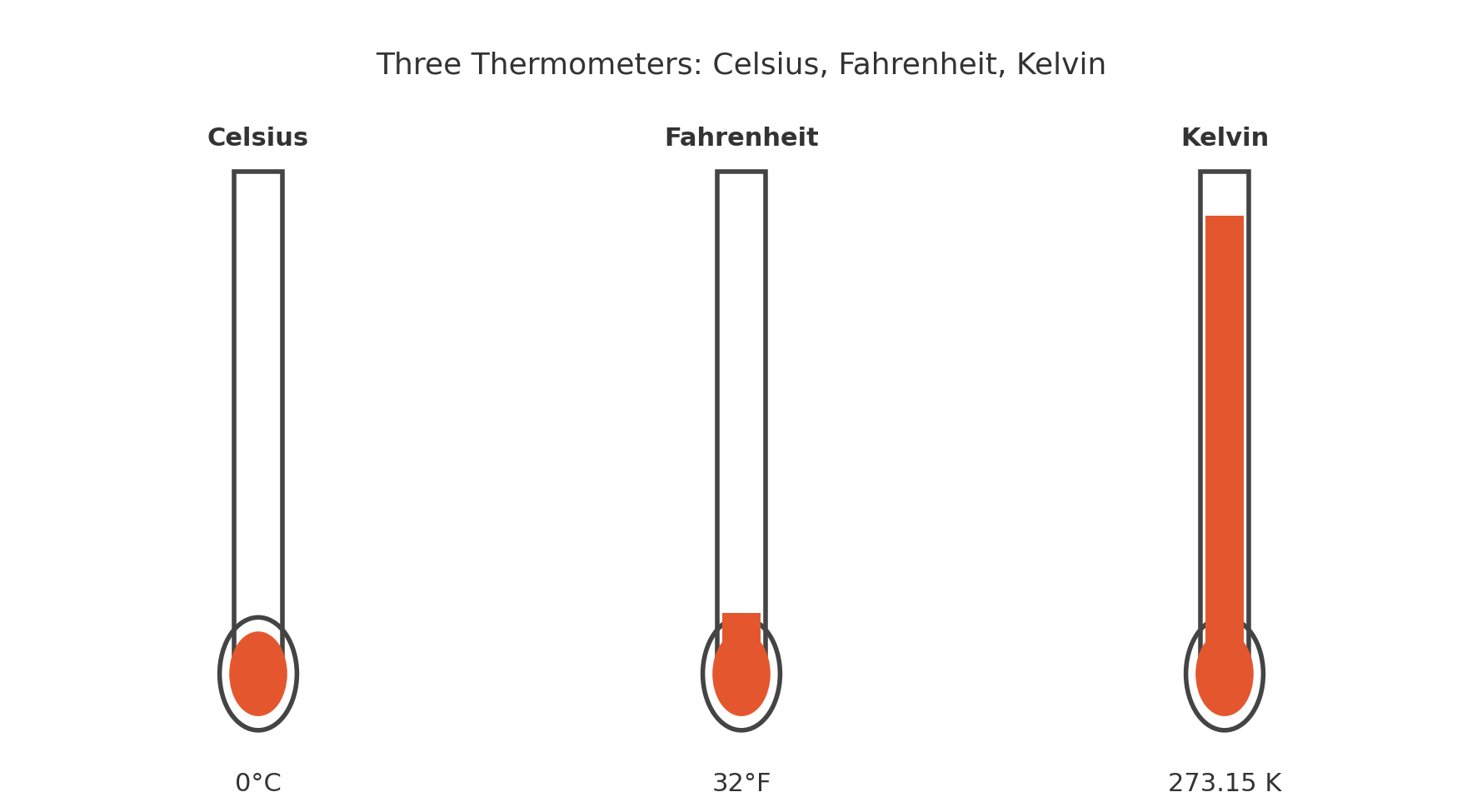
C, F, K thermometers juxstaposed

Drama: The Frozen Lab

Midnight in a physics laboratory.
The digital clock glows blue against the stainless steel counters. A researcher leans over a glass chamber filled with swirling vapor. The temperature sensors hum quietly.

She adjusts a dial—then another. The vapor slows, the molecular motion within it decreasing. The digital display falls:
5 Kelvin… 3 Kelvin… 1 Kelvin…

Finally, the numbers stabilize.
0 Kelvin.

She looks up and whispers, “Nothing moves.”

For the first time, zero means nothing at all. No motion. No energy. Not “cold,” not “less heat”—but the absence of temperature itself.

In this moment, measurement meets reality. The number zero no longer stands as a symbol or label—it marks the true origin of what is measured.


From Story to Concept: The Ratio Scale

In advanced sciences such as physics, measurement itself becomes a science.
When physicists speak of zero, they do not mean “a small number.” They mean the absence of what is measured.

Zero degrees on the Kelvin scale corresponds to the total absence of molecular motion, because temperature, in physical terms, is molecular motion.
At 0 K, nothing moves.

The ratio scale of measurement resembles the interval scale—equal distances between numbers—but goes further.
Here, zero is not arbitrary. It represents the true zero point in the phenomenon being measured.

With this foundation, we can now perform every mathematical operation:

  • Addition and subtraction (differences between quantities)
  • Multiplication and division (ratios, proportions, rates)

In ratio measurement, numbers are not merely symbolic; they are structural reflections of reality.
They allow science to speak in the language of law and proportion.

The ratio scale is the pinnacle of measurement:
zero becomes origin, and quantity becomes truth.

Practice self-test quiz

In the space below, please find practice problems and self-test quizzes. For full access, please signup free.

Story 4 — The Interval Scale of Measurement

The Interval Scale of Measurement

Drama: The Cold Morning

It’s a winter morning in New York. You wake up, open your phone, and check the weather. It says 32°F.
You sigh, grab your coat, and head out. The air bites your face.

By the time you reach the subway, your phone says 31°F. You frown. Has it really changed that much? You shrug.
Then you remember your cousin in Los Angeles posted a photo this morning: 62°F and sunny.

You type quickly:

“Hey, you’re twice as warm as I am!”

Then you stop. Something feels wrong.
Can 62 really be twice as warm as 31?
It feels like it, but you know it’s not true.

Later, in class, your statistics instructor confirms it:

“Temperature in Fahrenheit is interval, not ratio**.** You can add and subtract, but you can’t multiply or divide meaningfully. There’s no true zero—no absolute absence of heat.”

You smile. The world feels slightly warmer already.


From Story to Concept: The Interval Scale

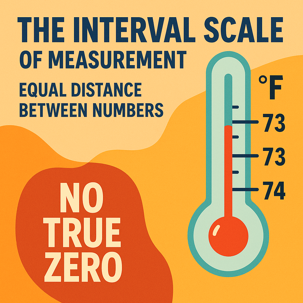
In the interval scale, the distance between numbers is equal.
Between 72 and 73 degrees Fahrenheit, the difference is the same as between 73 and 74.
You can even express subdivisions—72.4, 72.6—with equal precision.

This scale has a clear advantage over the nominal and ordinal types:
you can now perform addition and subtraction, and, in practice, even averages and standard deviations make sense.

However, one key element is missing: a true zero point.
Zero degrees Fahrenheit doesn’t mean no temperature; it simply marks an arbitrary point on the scale.

So while the interval scale lets you measure and compare distances precisely, it cannot meaningfully express ratios.
You can say it’s 10 degrees warmer today than yesterday—but not that it’s twice as warm.

The interval scale is a triumph of human thought—measurement without absolutes, order with equal steps but no foundation.


Practice self-test quiz

In the space below, please find practice problems and self-test quizzes. For full access, please signup free.

Story 3 — The Ordinal Scale of Measurement

The Ordinal Scale of Measurement99

Drama: Who’s Bigger

Twenty-first century Athens.
Today is the women’s Marathon.

Before you leave home, you catch a glimpse of the start line on television. The runners are ready in Marathon, the historic starting point. The finish line, as always, is the grand stadium in downtown Athens—the same place where the ancient games once ended.

You return home at dinner time. The family is gathered around the television, watching the news. Three winners stand proudly on the podium as the national anthems play.

“Great athletes!” you say.

Your family bursts into laughter.

“What’s so funny?” you ask. “Did I say something wrong? That was a great race—especially in this city’s smog!”

They laugh even harder. Finally, your father explains.

“The first runner truly was great—she broke the world record. But the second also broke the world record, only in a negative sense. She took so long to finish that no one in recorded history has ever taken that long. The smog made all the runners faint!”


From Story to Concept: The Ordinal Scale

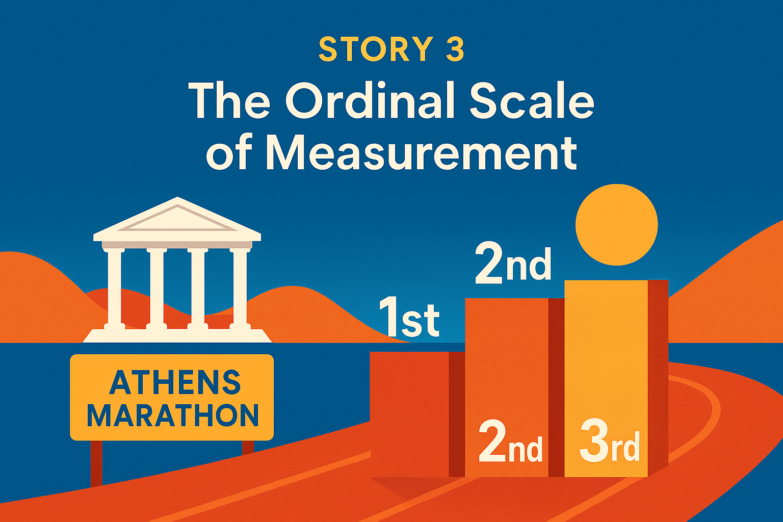
This type of measurement has an advantage over the nominal scale: it tells you which element is greater or lesser.
It introduces order.

You can now say who finished first, second, and third.
But you still don’t know by how much they differ.

The ordinal scale gives you ranking, not magnitude.
It answers which is greater, but not how much greater.

You cannot add, subtract, multiply, or divide ordinal numbers. You cannot calculate means or standard deviations. You cannot run sophisticated statistical analyses.

The ordinal scale is, in its essence, primitive—but revolutionary. It marks humanity’s first attempt to compare, to arrange, to impose order on experience.

It is the bridge between naming and measuring.

Practice self-test quiz

In the space below, please find practice problems and self-test quizzes. For full access, please signup free.

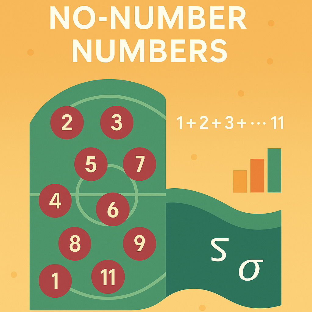
Story 2 — No-Number Numbers

Nominal numbers

It’s a Saturday afternoon on a soccer field in New York.
You’re sitting in the stands with your friends, pretending to enjoy the game. The truth is, you’re not much of a soccer fan. You open your laptop and drift into your own world.

Your friends are shouting and jumping with excitement. You, on the other hand, are studying the players.
You notice the numbers on their shirts.

“Hey,” you say, “who’s the guy with the number 11? He must be the best on the team. Poor number 3—he’s probably one of the worst.”

Your friends give you a look that says, please stop talking.

Unbothered, you go further:
“Guys, if you add up all the numbers on their shirts—1 + 2 + 3 + 4 + 5 + 6 + 7 + 8 + 9 + 10 + 11—it’s 66!”

You grin, waiting for applause.

Nothing.

So you take it up a notch.
You open your laptop, punch in the numbers, and announce proudly,
“I just calculated the standard deviation of the team’s jersey numbers!”

You never finish your sentence.
Your friends grab you, laughing, and shove you gently into the aisle.


From Story to Concept: The Ordinal Scale

The story of the soccer field is about numbers that aren’t really numbers.
The digits on the players’ shirts don’t measure anything. They only distinguish. Number 11 isn’t better than number 3, and adding 8 and 9 doesn’t produce a meaningful 17.

These are nominal numbers—they serve as labels, not quantities.
But we’re about to move one step further, to the next great human leap: the moment when order enters the world of measurement.

Practice self-test quiz

In the space below, please find practice problems and self-test quizzes. For full access, please signup free.


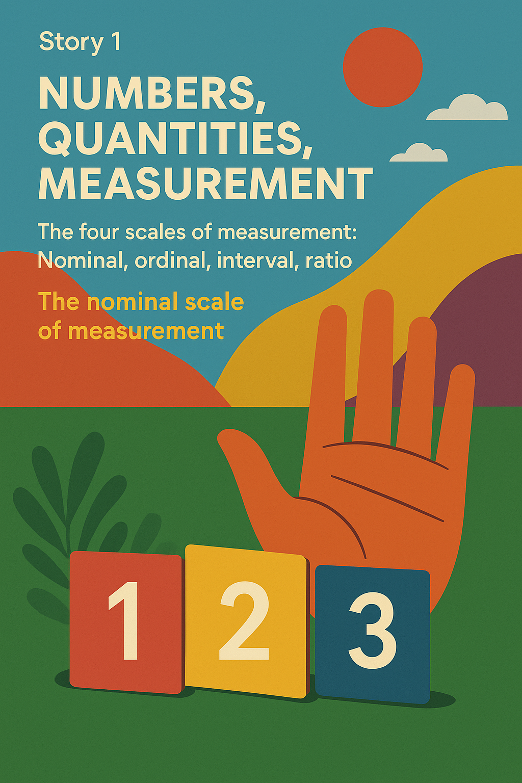
Story 1 — Numbers, Quantities, Measurement

Nominal scale of measurement

The Four Scales of Measurement

Nominal, ordinal, interval, ratio.
The first story belongs to the nominal scale—the simplest, and the oldest.


Drama: My Kids, My Fingers

A family of early Homo sapiens sits around a fire in a cave in Africa, devouring the evening meal of a goat-like animal. The children dance and chase each other; the women laugh and talk. The man stares into the dark mouth of the cave.

Now he raises his hands before his eyes. With the index finger of his right hand, he touches each finger of his left—one by one—his gaze fixed on his children. One child, one finger. He repeats the ritual with his other hand.

The next morning, he is crouched in the brush, waiting for game to pass. Again, he looks down at his hands. His eyes move from finger to finger—and he smiles. He knows how many children he has.

No words, no symbols. Only the raw sense of how many. The first pulse of number—the intuition of quantity—is born.

Thousands of years later, the names of each finger will no longer name a child but will stand for frequency, count, occurrence. They will become symbols: words like one, two, three.

And much later still, the words themselves will take form as written marks:
1, 2, 3.

Primitive arithmetic, yes—but also the first spark of the human mind’s most powerful invention: measurement.


From Story to Concept: The Nominal Scale

The man in the cave did not yet know numbers.
What he had discovered was naming.

He had no word for “one,” “two,” or “three.” But he knew this child and that child.
He separated—distinguished—each entity in his world. His perception of difference was the first act of measurement.

The nominal scale is born from that primitive gesture: the act of naming things to make them distinct.
It is the simplest form of measurement—no order, no magnitude, no arithmetic.

When we assign labels such as male and female, red and blue, apple and pear, we are using the nominal scale. These names carry identity but not quantity.
They answer the question what, not how many or how much.

In the story, each finger represented a child—not a number, but a name, a mark of uniqueness. The father’s counting was not numerical; it was symbolic, categorical. He was labeling, not adding.

Later in history, this act of naming evolved into words that expressed magnitude—one, two, three.
But before there were numbers, there were names.
And before there was mathematics, there was distinction—the mind’s first measurement of the world.

Practice self-test quiz

In the space below, please find practice problems and self-test quizzes. For full access, please signup free.
Part 8 --- The Storyteller Statistician

The storyteller statistiian

Part 7: The Storyteller Statistician

Think statistics means scary formulas and endless algebra? Think again.

In this part you only need everyday arithmetic: addition, subtraction, multiplication, and division. Most formulas are written in plain words rather than symbols — and you really only need to master one core idea.

This book is designed for high school students heading toward college science majors (and anyone who wants to understand statistics in the real world). Few high school textbooks cover so many statistical tests — and even fewer explain complex designs such as mixed or split-plot ANOVA, which can feel truly challenging but rewarding.

What sets this resource apart is its focus on real-life application. Most people use statistics in practical research, not in abstract mathematics. Learning to plug numbers into complicated equations is useful, but it is not enough. Real understanding comes from experience in actual research settings — exactly what these stories aim to build.

Stories in Part 7

Complete list of stories

  • Story 1 — Numbers, Quantities, Measurement How we turn observations into numbers we can trust.
  • Story 2 — No-Number Numbers When "numbers" are really categories or ranks.
  • Story 3 — The Ordinal Scale of Measurement Ranking things without assuming equal intervals.
  • Story 4 — The Interval Scale of Measurement Equal differences that still lack a true zero.
  • Story 5 — My Zero Is Not Zero Why zero can be arbitrary — and what that means for data.
  • Story 6 — The Goddess Normal Curve Why the bell curve appears everywhere — and how to use it wisely.
  • Story 7 — Variance and Standard Deviation Measuring how spread out your data really is.
  • Story 8 — The Uses of the Normal Distribution Everyday applications beyond the basics.
  • Story 9 — Normal Distribution: Use #1 — Describing and Organizing Data Using the curve to summarize and compare groups.
  • Story 10 — Normal Distribution: Use #2 — Making Statements of Probability and Betting Turning the curve into probabilities for decisions and risks.
  • Story 11 — Normal Distribution: Use #3 — Reliability of a Single Mean Confidence intervals for one group's average.
  • Story 12 — Normal Distribution: Use #4 — Reliability of the Difference Between Two Means Comparing groups with statistical confidence.
  • Story 13 — The t-test The go-to test when samples are small or variance unknown.
  • Story 14 — An Example of the t-test A step-by-step real-world application.
  • Story 15 — Analysis of Variance: One-Way ANOVA Comparing means across more than two groups.
  • Story 16 — Analysis of Variance: Factorial Designs Testing multiple factors and their interactions at once.
  • Story 16A — Example of a 2×2 Factorial Experiment A concrete look at two factors interacting.
  • Story 16B — Example 2 of a 2×2 Factorial Experiment Another practical illustration of interactions.
  • Story 17 — Example of a 2×3 Factorial Experiment Expanding to more levels for richer insights.
  • Story 18 — Repeated-Measures ANOVA Analyzing the same subjects over time or conditions.
  • Story 19 — Complex, Mixed, Split-Plot Designs (ANOVA) Handling advanced, real-world experimental structures.

These stories take you from basic measurement to advanced ANOVA designs — all told through real-world examples and simple reasoning. Start wherever you like, or follow the sequence in the book navigation. Which story surprises you most? Share your thoughts in the comments below!