Lecture 5 — The t-test

t-test independence
paired treatments
t-pairded
t z

This lecture emphasizes conceptual understanding of the t-test, its logic, and how it fits into the broader structure of statistical reasoning.

The t-test is one of the most widely used statistical tools.
It compares two means and asks: Is the difference between them real, or could it be due to chance?

The t-test is closely related to the z-test.
When the population standard deviation is unknown and the sample size is small, we use t instead of z.


Types of t-Tests

  • One-sample t-test: compares a sample mean to a known or hypothesized population mean.
  • Independent-samples t-test: compares means from two separate groups.
  • Paired-samples t-test: compares two scores from the same group (before vs. after).

Symbolic Formulas

One-sample t-test
$$t = \frac{\bar{X} - \mu_0}{s / \sqrt{n}}$$

Independent-samples t-test
$$t = \frac{\bar{X}_1 - \bar{X}_2}{\sqrt{\tfrac{s_1^2}{n_1} + \tfrac{s_2^2}{n_2}}}$$

Paired-samples t-test
$$t = \frac{\bar{D}}{s_D / \sqrt{n}}$$


Degrees of Freedom

  • One-sample: $$df = n - 1$$
  • Independent-samples: $$df = n_1 + n_2 - 2$$
  • Paired-samples: $$df = n - 1$$

Example (Independent t-Test)

Two groups of students try different study methods:

  • Group A: \(n = 10\), mean = 80, SD = 10
  • Group B: \(n = 10\), mean = 90, SD = 10

$$t = \frac{80 - 90}{\sqrt{\tfrac{10^2}{10} + \tfrac{10^2}{10}}} = \frac{-10}{\sqrt{10 + 10}} = \frac{-10}{\sqrt{20}} = \frac{-10}{4.47} = -2.24$$

Degrees of freedom = 18.
Compare this t-value to the critical value in the t-table at \(df = 18\).


Example (Paired t-Test)

Students take a test before and after tutoring.
Differences (After − Before): 4, 6, 5, 3, 2.

Mean difference:
$$\bar{D} = \frac{4 + 6 + 5 + 3 + 2}{5} = 4$$

Standard deviation of differences:
$$s_D = 1.58$$

$$t = \frac{4}{1.58 / \sqrt{5}} = \frac{4}{0.71} = 5.63$$

Degrees of freedom = 4.
This large t-value indicates strong evidence of improvement.


Definition

  • Independent t-test: compares two separate groups.
  • Paired t-test: compares the same group measured twice.
  • Degrees of freedom (df): number of independent pieces of information.

Visuals

Figure L5.1 — Independent t-Test. Bar graph of two groups (A and B) with means and SEM error bars.

Figure L5.2 — Paired t-Test. Line plot showing before vs. after scores for each student.

Figure L5.3 — t vs. z Distribution. Overlay of the normal (z) curve and t curves with df = 5 and 20.


Why This Matters

The t-test is the workhorse of statistics.
It forms the foundation for many other methods (ANOVA, regression, mixed models).
Understanding t means understanding how we compare signal (mean difference) to noise (variability).

Practice self-test quiz

In the space below, please find practice problems and self-test quizzes. For full access, please signup free.
Lecture 4 — Uses of the Normal Distribution

two normal curves

The normal distribution is not just a shape — it is a powerful tool.
It allows us to describe data, calculate probabilities, and make decisions about means and differences.

Here are four major uses of the normal curve.


1. Describing Data

The normal curve summarizes how scores are distributed.

  • Mean = center
  • Standard deviation = spread

It provides a reference point: where most scores fall, and where extremes occur.

Figure L4.1 — Normal Curve with mean and ±1σ, ±2σ, ±3σ marked.


2. Probability of a Score

We can use the normal curve to calculate the probability of observing a score above or below a certain value.

Formula for standardization:
$$z = \frac{x - \mu}{\sigma}$$

Formula in words:
$$z = \frac{\text{score} - \text{mean}}{\text{standard deviation}}$$

The z-score tells us how many standard deviations a score is from the mean.
With the z-table, we can find the probability of that score.

Figure L4.2 — Normal curve with shaded area above z = 1.5.


3. Reliability of a Mean (SEM)

If we take many samples, the means vary. The Standard Error of the Mean (SEM) tells us how much.

Formula:
$$\mathrm{SEM} = \frac{s}{\sqrt{n}}$$

Formula in words:
$$\text{SEM} = \frac{\text{standard deviation}}{\sqrt{\text{number of scores}}}$$

Smaller SEM means the sample mean is a more reliable estimate of the population mean.

Figure L4.3 — Distribution of sample means, narrower than distribution of raw scores.


4. Reliability of a Difference

The normal distribution also underlies hypothesis testing — such as the t-test.
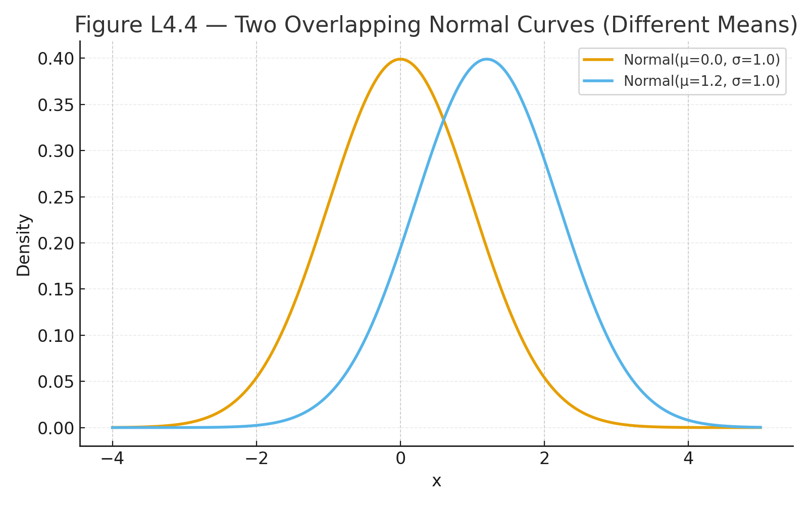
It allows us to compare two means and decide whether their difference is larger than expected by chance.

Figure L4.4 — Two overlapping normal curves with different means.


Why This Matters

The normal distribution is the foundation for:

  • Calculating probabilities
  • Estimating reliability of means
  • Testing hypotheses about differences

Understanding these uses prepares us for the transition from descriptive to inferential statistics.

Practice self-test quiz

In the space below, please find practice problems and self-test quizzes. For full access, please signup free.
Lecture 3 — Variance & Standard Deviation

variability

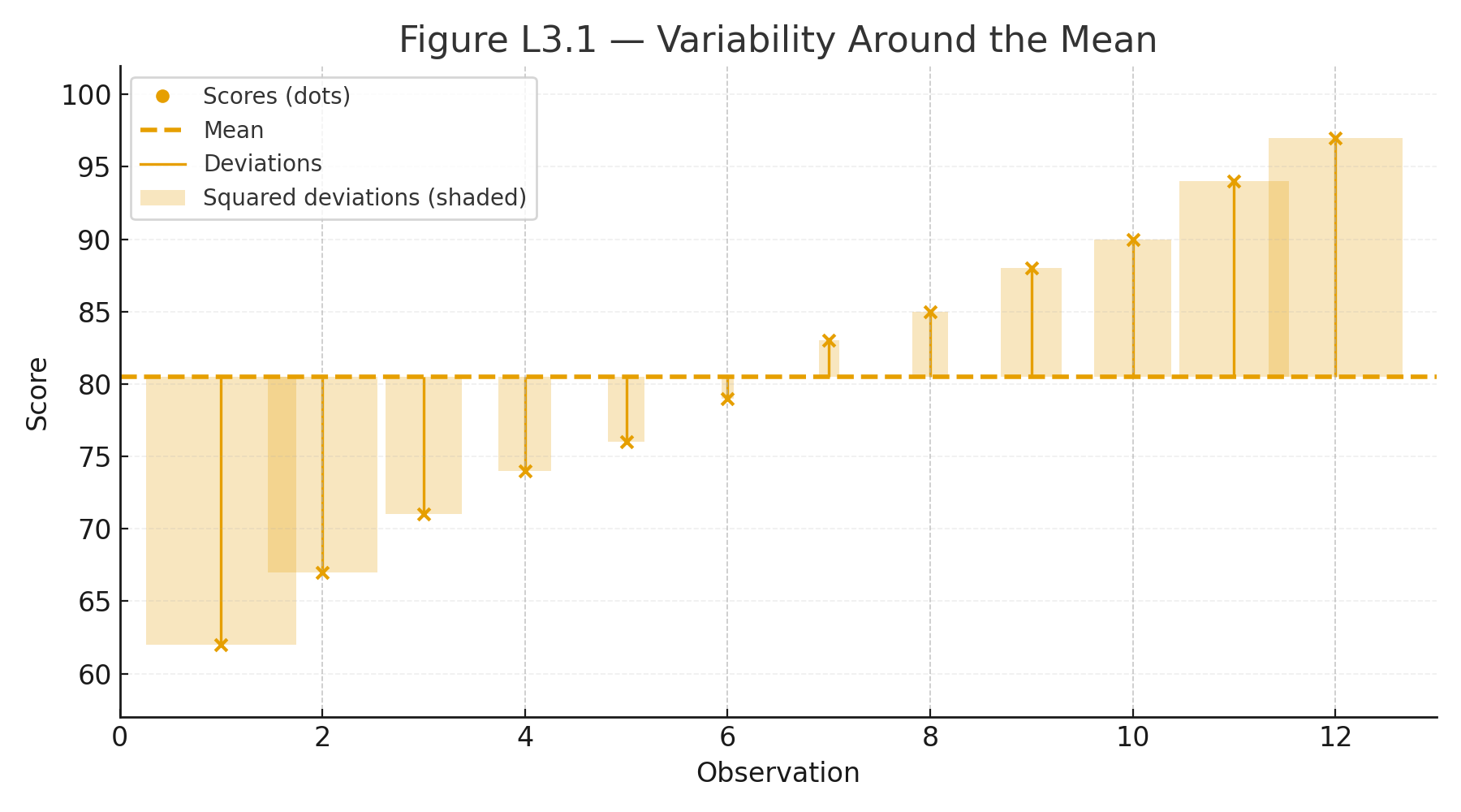
The mean tells us the “typical” score. But how tightly do scores cluster around the mean? Do they spread widely, or are they close together?

To answer, we measure variability. Two key measures are the variance and the standard deviation.


Variance

Variance is the average squared distance of scores from the mean.

Symbolic formula:
$$s^2 = \frac{\sum (X - \bar{X})^2}{n - 1}$$

Formula in words:
$$\text{Variance} = \frac{\text{sum of squared deviations from the mean}}{\text{number of scores} - 1}$$

Where:

  • $$s^2$$ = variance
  • $$X$$ = each score
  • $$\bar{X}$$ = mean
  • $$n$$ = number of scores

Standard Deviation

The standard deviation is the square root of the variance. It puts variability back into the same units as the data.

Symbolic formula:
$$s = \sqrt{\frac{\sum (X - \bar{X})^2}{n - 1}}$$

Formula in words:
$$\text{Standard deviation} = \sqrt{\frac{\text{sum of squared deviations from the mean}}{\text{number of scores} - 1}}$$


Example

Data: 6, 8, 10

  • Mean = 8
  • Deviations: –2, 0, 2
  • Squared deviations: 4, 0, 4
  • Sum = 8

Variance:
$$s^2 = \frac{8}{3-1} = 4$$

Standard deviation:
$$s = \sqrt{4} = 2$$

So, on average, scores are 2 units away from the mean.


Definition

  • Variance: average squared distance from the mean.
  • Standard Deviation: square root of variance; typical distance from the mean.

Visuals

Figure L3.1 — Variability Around the Mean. Dot plot of scores with the mean marked, vertical lines for deviations, and shaded boxes for squared deviations.


Why This Matters

Two sets of scores can have the same mean but very different spreads.
Variance and standard deviation give us the language to describe spread, and they are the building blocks for t-tests, ANOVA, and all inferential statistics.

Practice self-test quiz

In the space below, please find practice problems and self-test quizzes. For full access, please signup free.
Lecture 2 — The Goddess Normal Curve

normal curve
normal curvre 68 95
z score 1.0

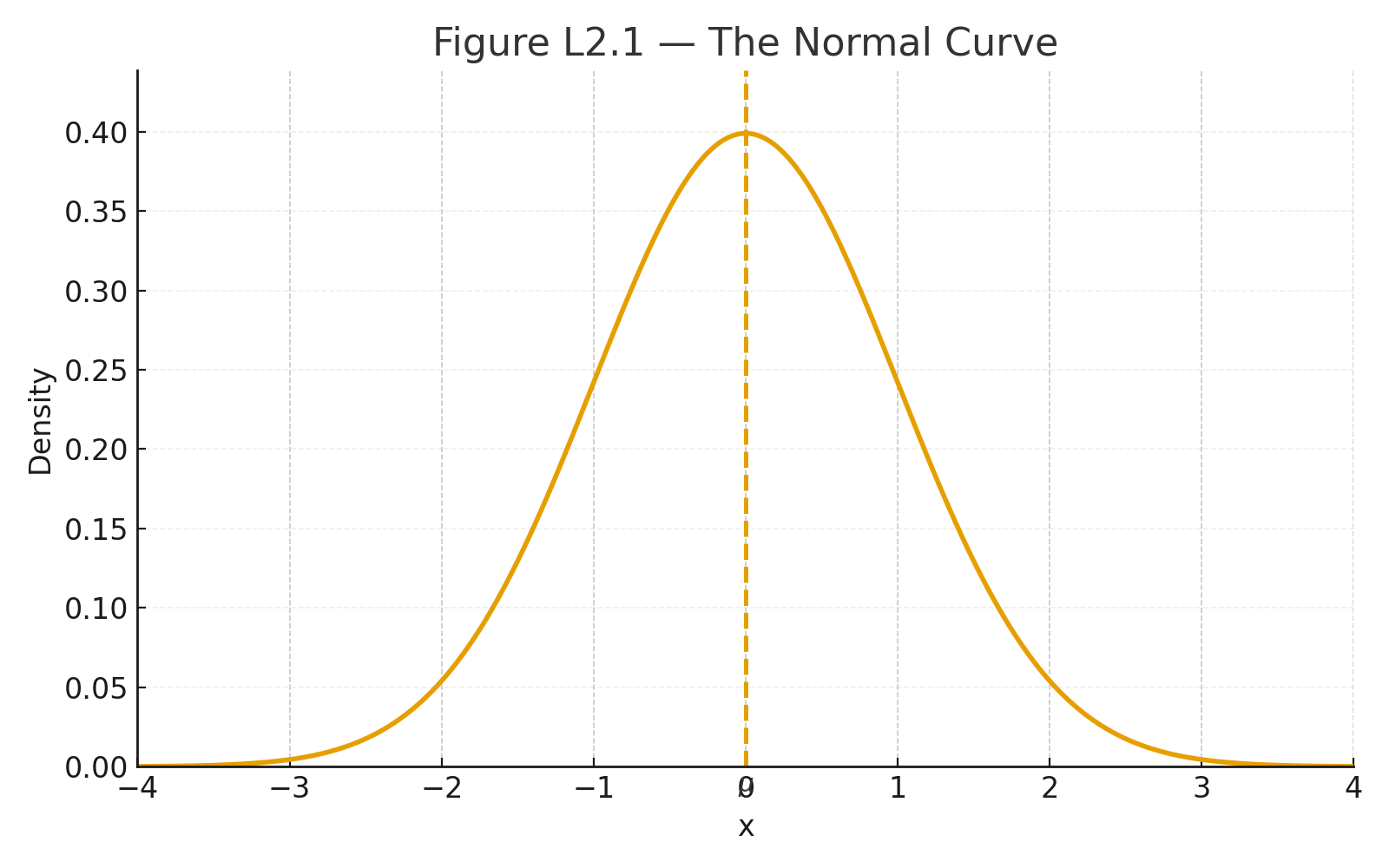
The normal curve (bell curve) is one of the most important concepts in statistics.
It is elegant, symmetrical, and central to probability and inference.
It appears whenever many small, independent factors combine: height, exam scores, measurement errors.


Properties of the Normal Curve

  1. Symmetrical around the mean
  2. One peak (unimodal)
  3. Mean = Median = Mode
  4. Total area under the curve = 1 (100%)

Formula for the Normal Distribution

Symbolic formula:
$$f(x) = \frac{1}{\sigma \sqrt{2\pi}} e^{-\frac{(x - \mu)^2}{2\sigma^2}}$$

Formula in words:
$$\text{Probability density} = \frac{1}{\text{standard deviation} \times \sqrt{2\pi}} \times e^{-\frac{(\text{score} - \text{mean})^2}{2 \times (\text{standard deviation})^2}}$$

Where:

  • $$\mu$$ = mean
  • $$\sigma$$ = standard deviation
  • $$x$$ = a score

Standardization (z-scores)

Symbolic formula:
$$z = \frac{x - \mu}{\sigma}$$

Formula in words:
$$z = \frac{\text{score} - \text{mean}}{\text{standard deviation}}$$

A z-score tells us how many standard deviations a score is above or below the mean.


Key Percentages

Under the normal curve:

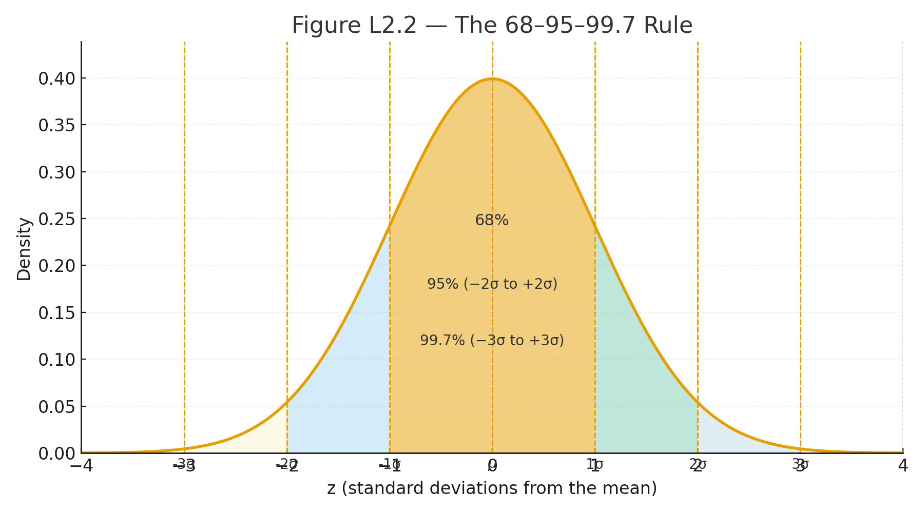
  • About 68% of scores are within 1 standard deviation of the mean
  • About 95% are within 2 standard deviations
  • About 99.7% are within 3 standard deviations

This is called the 68–95–99.7 rule.


Drama Box — “The Goddess Normal Curve”

Imagine a temple where a perfect curve stands tall — balanced and symmetrical.

  • At the center is the mean, the balance point.
  • Half of the people (data) stand on each side.
  • As you move further away, fewer remain.
  • The Goddess teaches fairness: most scores are near the center, extreme scores are rare.

This image helps students remember the normal curve not as a dry formula, but as a principle of balance and probability.


Visuals

Figure L2.1 — The Normal Curve. Bell-shaped curve centered at the mean (μ).

Figure L2.2 — The 68–95–99.7 Rule. Normal curve with shaded regions ±1σ, ±2σ, ±3σ.

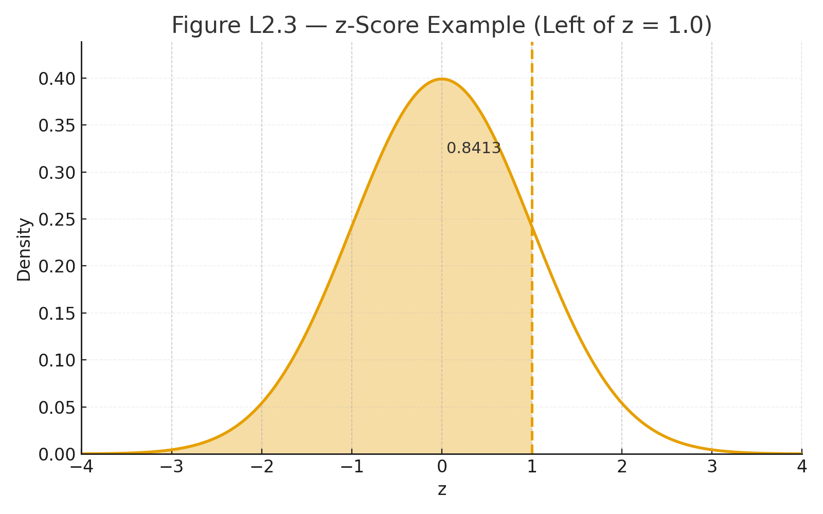
Figure L2.3 — z-score Example. Normal curve with shaded area to the left of z = 1.0, labeled 0.8413.


Why This Matters

The normal curve is the foundation of inferential statistics.

  • It allows us to calculate probabilities.
  • It underlies t-tests, ANOVAs, and confidence intervals.
  • It lets us compare scores across different tests and scales.

Practice self-test quiz

In the space below, please find practice problems and self-test quizzes. For full access, please signup free.
Lecture 1 — Scales of Measurement

scales of measurement

Before we can analyze data, we must know how it was measured.
The type of measurement determines which statistical test is appropriate.

Scientists and psychologists classify data into four scales of measurement: nominal, ordinal, interval, and ratio.


The Four Scales

  1. Nominal Scale
    • Numbers are just labels or categories.
    • Example: 1 = Male, 2 = Female.
    • No arithmetic can be done.
  2. Ordinal Scale
    • Numbers show order or rank, but not equal intervals.
    • Example: 1st place, 2nd place, 3rd place.
    • We know who is higher, but not by how much.
  3. Interval Scale
    • Numbers have equal intervals, but no true zero.
    • Example: Temperature in °C.
    • 20°C is warmer than 10°C, but not “twice as hot.”
  4. Ratio Scale
    • Numbers have equal intervals and a true zero.
    • Example: Height, weight, reaction time.
    • Ratios are meaningful: 20 kg is twice 10 kg.

Definition

  • Nominal: categories only
  • Ordinal: rank order
  • Interval: equal intervals, no true zero
  • Ratio: equal intervals, true zero

Drama Box — “My Kids, My Fingers”

A professor once explained measurement scales by holding up his hand.

  • “I have five fingers. That’s a ratio scale — it’s a real count, and zero means none.”
  • “If I say this finger is first, that’s an ordinal scale.”
  • “If I call them One, Two, Three, that’s just labels — a nominal scale.”
  • “If I measure temperature in Celsius on my skin, that’s interval — the numbers are spaced evenly, but zero doesn’t mean no heat.”

The story helps students remember: labels, ranks, intervals, ratios — the four levels of measurement.


Visuals

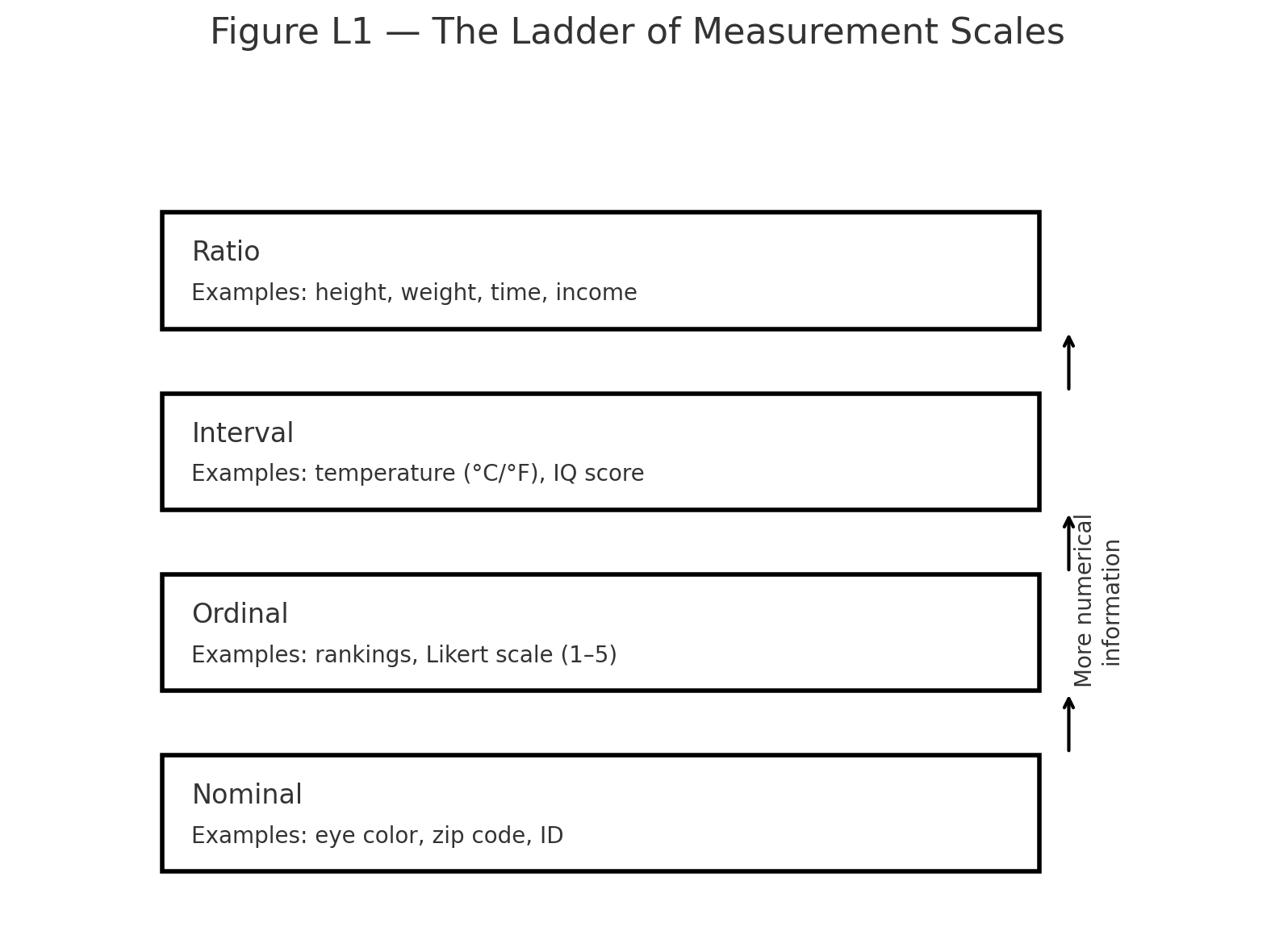
Figure L1 — The Ladder of Measurement Scales. Four rungs labeled: Nominal → Ordinal → Interval → Ratio, each with examples.


Why This Matters

  • Nominal/Ordinal data → non-parametric tests
  • Interval/Ratio data → parametric tests

This decision is the first step in statistics.
Before calculating a mean, a t-test, or an ANOVA, we must ask: How were the data measured?

Practice self-test quiz

In the space below, please find practice problems and self-test quizzes. For full access, please signup free.
Lesson 8 — Post Hoc Tests

tukey hsd
bonferroni

When ANOVA finds a significant F, we know that not all group means are equal.
But ANOVA does not tell us which groups differ.

For that, we need post hoc tests (Latin: after this).
They compare pairs of group means while controlling for the increased chance of error.


Tukey’s Honestly Significant Difference (HSD)

When to Use:

  • Equal group sizes
  • Pairwise comparisons after one-way ANOVA

Formula:
$$\text{HSD} = q \sqrt{\frac{MS_{\text{within}}}{n}}$$

In words:
$$\text{HSD} = \text{Studentized range statistic } q \times \sqrt{\frac{\text{mean square within groups}}{\text{sample size per group}}}$$

If the difference between two means ≥ HSD, they are significantly different.

Example:
3 groups, n = 10 each, $$MS_{\text{within}} = 16.7$$, critical $$q = 3.5$$.

$$\text{HSD} = 3.5 \times \sqrt{\tfrac{16.7}{10}} = 3.5 \times 1.29 = 4.52$$

So any pair of means that differ by 4.52 or more is significant.


Bonferroni Correction

When to Use:

  • Simple and conservative
  • Divide significance level by number of comparisons

Formula:
$$\alpha' = \frac{\alpha}{m}$$

In words:
$$\text{adjusted significance level} = \frac{\text{original significance level}}{\text{number of comparisons}}$$

Example: If α = 0.05 and 10 comparisons, α′ = 0.005 per test.


Scheffé Test

When to Use:

  • Unequal sample sizes
  • Often highly conservative for pairwise comparisons and protective of all possible contrasts

Formula (summary):
Scheffé’s critical F = (k – 1) × F(critical, df_between, df_within).


Definition

  • Post hoc test: statistical test used after ANOVA to identify which means differ
  • Tukey HSD: balanced groups, pairwise
  • Bonferroni: adjusts α for multiple comparisons
  • Scheffé: conservative, flexible for unequal n

Visual Placeholders

Figure 8.1 — Tukey HSD example: three group means with horizontal bars showing which pairs differ.

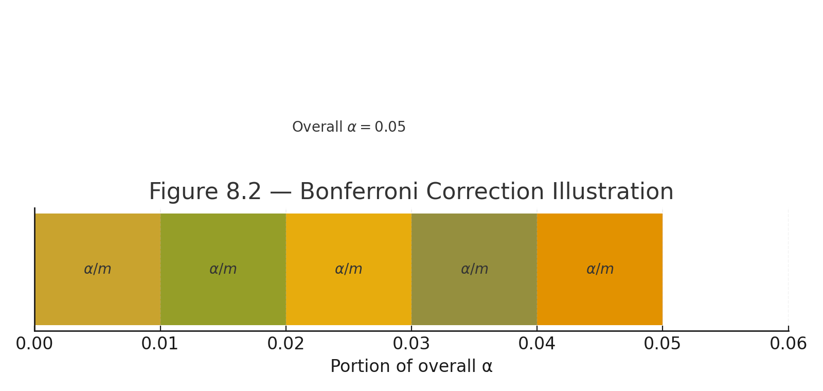
Figure 8.2 — Bonferroni correction illustration: α = 0.05 split into smaller pieces.


Why This Matters

ANOVA can indicate evidence of differences somewhere.
Post hoc tests examine specific comparisons.
They control the risk of false positives across multiple group comparisons.

Practice self-test quiz

In the space below, please find practice problems and self-test quizzes. For full access, please signup free.

Lesson 7 — Analysis of Variance (ANOVA)

anova layout
partitioning variance
2x2 factorial layout
factorial interaction
repeated measures anova
mixed anova layout
anova summary table

Lesson 7: Analysis of Variance (ANOVA)

The t-test is great for comparing two means. But what happens when you have three, four, or even more groups? Running multiple t-tests increases the chance of false positives (Type I error inflation). The solution is Analysis of Variance (ANOVA) — a powerful method that compares means across multiple groups in one test.

What ANOVA Does

ANOVA tests whether the means of several groups are significantly different from each other. It does this by partitioning (splitting) the total variability in the data into two parts:

  • Between-groups variability: Differences caused by the treatment or factor (the effect we care about).
  • Within-groups variability: Differences due to random chance or individual differences within each group (error or noise).

If between-groups variability is much larger than within-groups variability, the group means likely differ because of the treatment — not just chance.

The F Ratio — The Heart of ANOVA

The test statistic is the F ratio:

$$ F = \frac{MS_{\text{between}}}{MS_{\text{within}}} $$

In words:

$$ F = \frac{\text{Mean Square Between Groups}}{\text{Mean Square Within Groups}} $$

Where:

  • $$ MS_{\text{between}} = \frac{SS_{\text{between}}}{df_{\text{between}}} $$ (variance explained by the groups)
  • $$ MS_{\text{within}} = \frac{SS_{\text{within}}}{df_{\text{within}}} $$ (variance due to error)

A large F value suggests the between-groups differences are real, not random.

Degrees of Freedom in One-Way ANOVA

  • $$ df_{\text{between}} = k - 1 $$ (k = number of groups)
  • $$ df_{\text{within}} = N - k $$ (N = total number of observations)
  • $$ df_{\text{total}} = N - 1 $$

Example: One-Way ANOVA

Three groups of students use different study techniques:

  • Group A: mean = 70
  • Group B: mean = 75
  • Group C: mean = 85

Suppose calculations give:

  • $$ SS_{\text{between}} = 300 $$, $$ df_{\text{between}} = 2 $$ → $$ MS_{\text{between}} = 150 $$
  • $$ SS_{\text{within}} = 200 $$, $$ df_{\text{within}} = 12 $$ → $$ MS_{\text{within}} = 16.7 $$

Then:

$$ F = \frac{150}{16.7} \approx 9.0 $$

Compare F = 9.0 to the critical value from the F-table (df = 2, 12) ≈ 3.89 at p = 0.05. Since 9.0 > 3.89, the result is significant — the study techniques produce different mean scores.

Types of ANOVA

Factorial ANOVA

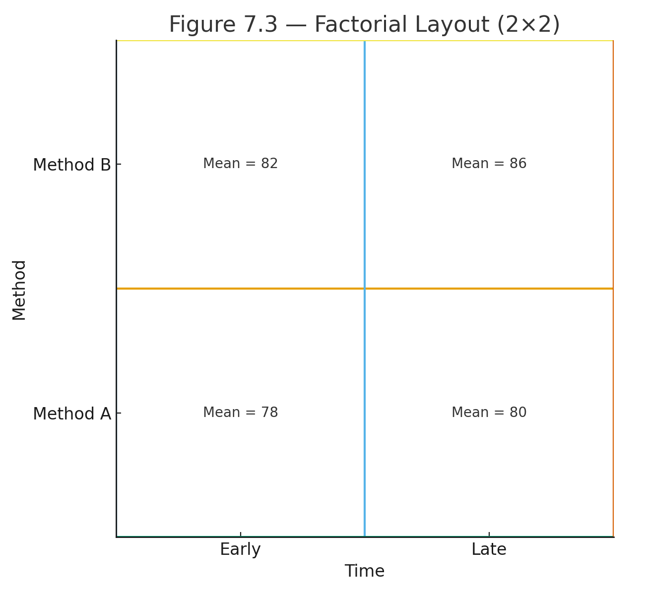
Tests two or more factors simultaneously (e.g., teaching method × time of day in a 2×2 design). It reveals:

  • Main effects of each factor
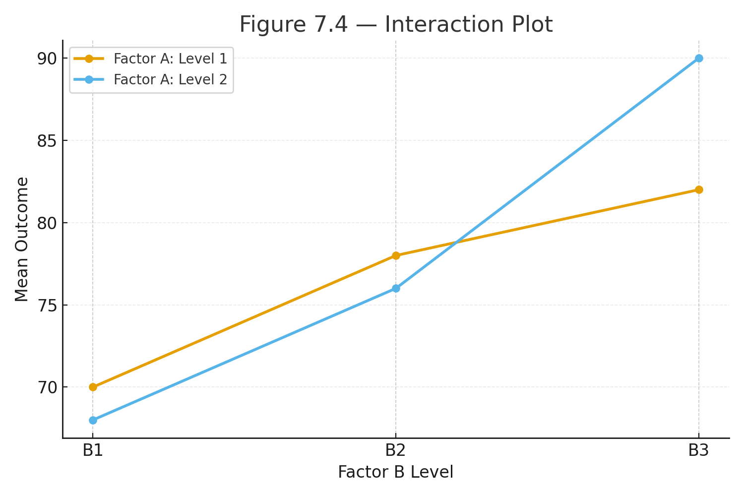
  • Interaction effects (when one factor's effect depends on the level of another)

Repeated-Measures ANOVA

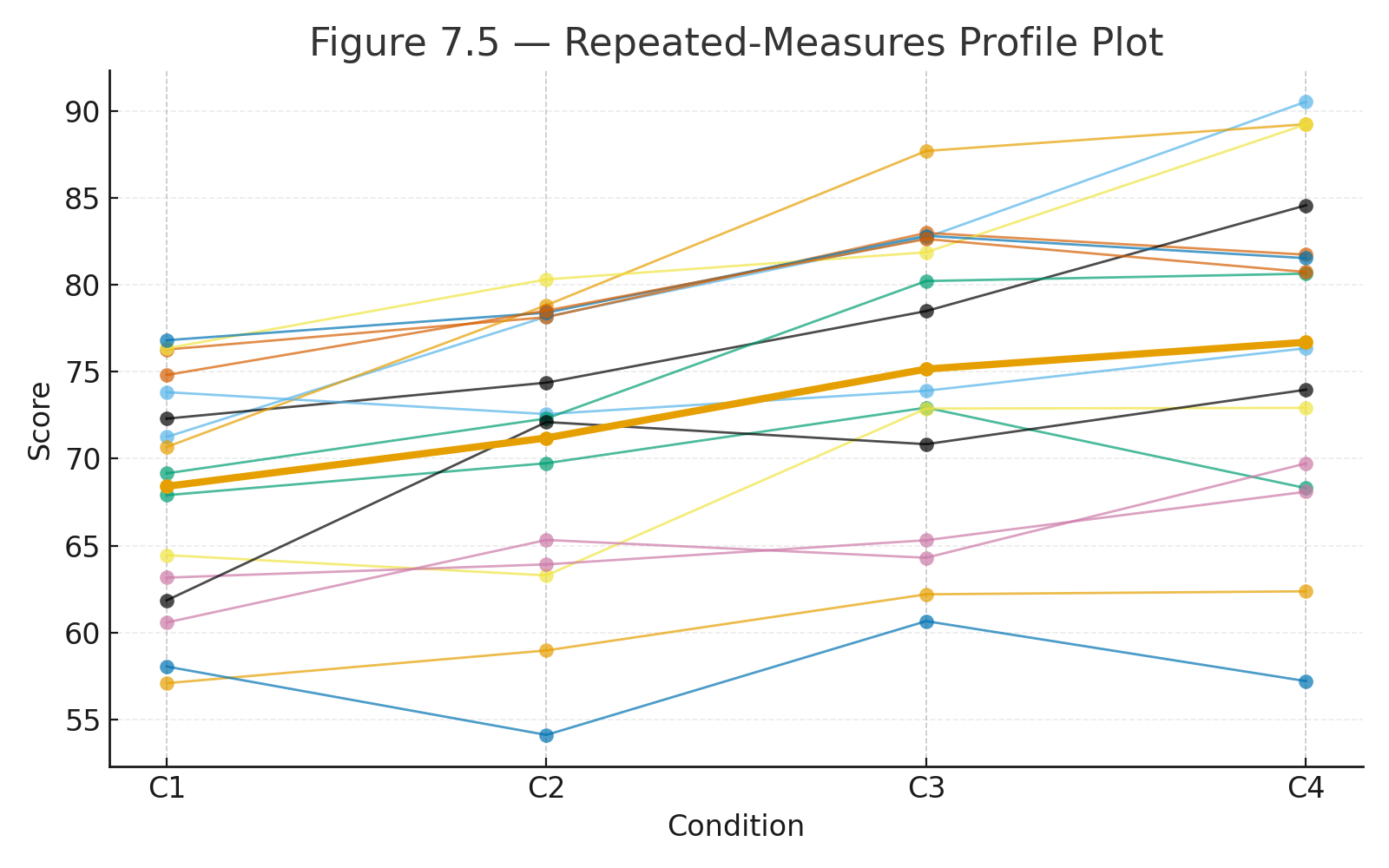
Used when the same participants are measured multiple times (e.g., test scores before, during, and after a treatment). Removes individual differences, increasing statistical power.

Mixed (Split-Plot) ANOVA

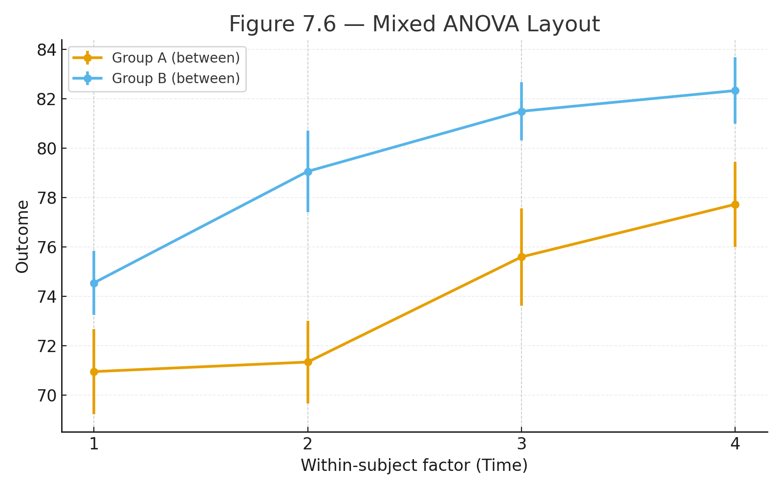
Combines between-subjects (e.g., different treatment groups) and within-subjects (e.g., repeated measures over time) factors. Common in psychology, education, and clinical research.

Quick Summary

  • ANOVA generalizes the t-test to 3+ groups.
  • F ratio compares explained variance to error variance.
  • Large F → likely real differences between groups.
  • Types: one-way, factorial, repeated-measures, mixed.

Visuals

Figure 7.1 — One-way ANOVA: Bar chart showing group means with error bars.

Figure 7.2 — Variance partitioning: Total SS split into Between SS and Within SS.

Figure 7.3 — 2×2 Factorial design grid.

Figure 7.4 — Interaction plot: Non-parallel lines indicate interaction.

Figure 7.5 — Repeated-measures profile plot.

Figure 7.6 — Mixed ANOVA structure.

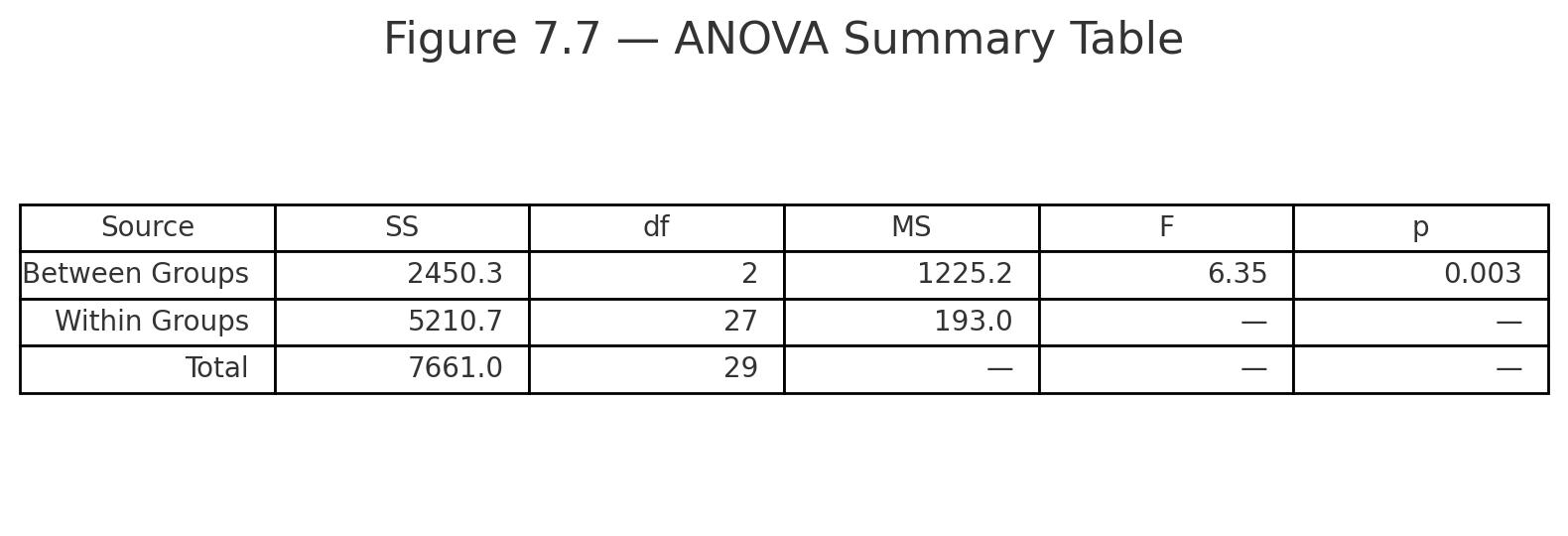
Figure 7.7 — Standard ANOVA summary table (Source | SS | df | MS | F | p).

Why ANOVA Matters

ANOVA is one of the most powerful and widely used tools in science. It helps researchers determine whether differences among groups are meaningful — not just random noise — making it essential for experiments in psychology, education, biology, medicine, and more.

Practice & Self-Test

Try the interactive self-test quiz below to check your understanding of ANOVA concepts, F ratio, and interpretation. For full access and more problems, sign up free.


Lesson 6 — The t-Test: Worked Examples & Calculations

t- one sample
t- one sample curve
t- independent boxplot
t- independent means
t- independent curve
t welch
t paired profile
t- paird curve
t-residuals

Introduction. This lesson is hands-on, data-driven, and calculation-oriented. It prepares students to do t-tests with data. The t-test compares means when the population standard deviation is unknown and is estimated from the sample, so the standardized statistic follows Student’s t distribution with appropriate degrees of freedom (df). The three common variants are: (a) one-sample (compare a sample mean to a reference value \( \mu_0 \)); (b) independent-samples (compare means of two unrelated groups); and (c) paired-samples (compare repeated measures on the same units by testing the mean of the differences). Classical t-tests assume independence at the relevant observational level and approximate normality of the observations, residuals, or paired differences, depending on the design; only the pooled independent-samples test assumes equal variances.


A) One-Sample t-Test

Goal. Test whether a sample mean differs from a known/reference mean \( \mu_0 \).

Design & Experiment

A company claims average battery life is \( \mu_0 = 10 \) hours. We test \( n=12 \) units.

Data

Hours (n = 12)
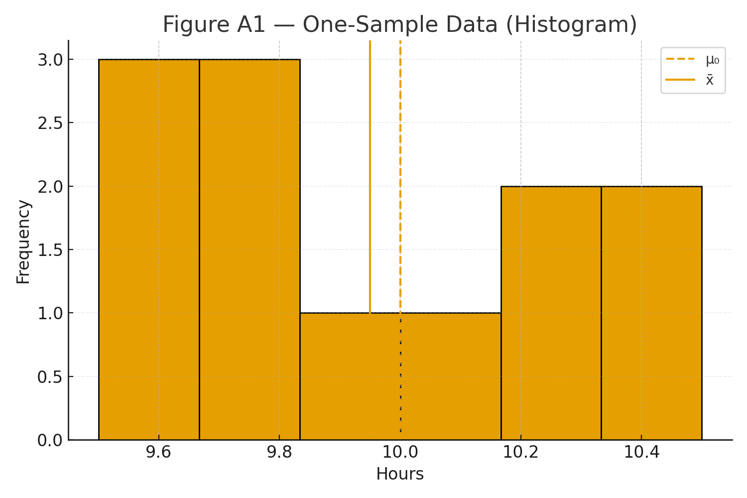
9.6, 10.1, 10.5, 9.9, 9.7, 10.4, 9.8, 9.6, 10.2, 9.5, 10.3, 9.8
Histogram of the twelve battery-life observations used in the one-sample t-test.
Figure A1: Histogram/QQ plot for one-sample data.

Step 1 — Sum, Mean, Variance

\(\sum x = 119.4 \Rightarrow \bar X = 9.95.\) Using \( \sum (x-\bar X)^2 = 1.270 \Rightarrow s^2 = 1.270/11 = 0.11545,\; s = 0.33979.\)

Step 2 — Test Statistic & p-value

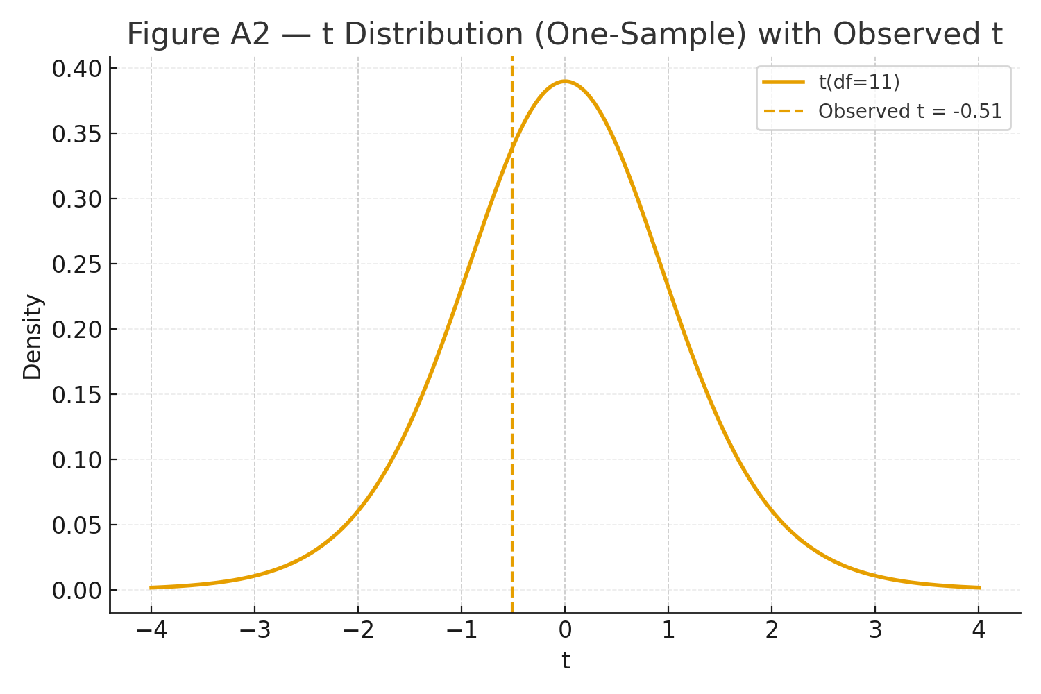
\(\displaystyle SE = \frac{s}{\sqrt{n}} = \frac{0.33979}{\sqrt{12}} = 0.09809,\quad t = \frac{\bar X - \mu_0}{SE} = \frac{9.95 - 10}{0.09809} = -0.50975,\quad df = n-1 = 11. \)

Two-tailed \(p \approx 0.6203\) → fail to reject \(H_0\).

Student t distribution with 11 degrees of freedom and the observed t statistic marked.
Figure A2: t curve (df=11) with observed \(t\) marked.

Conclusion (One-Sample)

No evidence the true mean differs from 10 hours (\(t(11)=-0.51,\; p=.620\)).


B) Independent-Samples t-Test

Goal. Test whether two teaching methods lead to different average exam scores.

Design & Experiment

Twenty students are randomly assigned to one of two methods (n = 10 per group).

  • Method A: Active discussion
  • Method B: Structured lecture

After a 2-week module, everyone takes the same 100-point exam.

Data

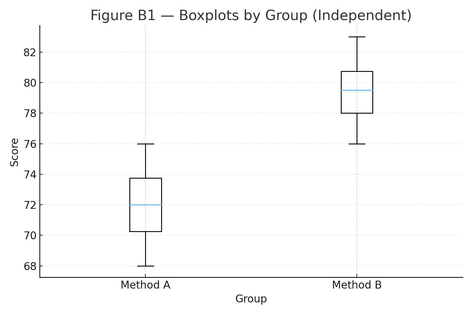
Method AMethod B
7278
6882
7580
7077
6979
7381
7183
7476
7678
7280
Boxplots comparing exam scores for teaching Methods A and B.
Figure B1: Boxplots of scores by group.

Step 1 — Sums & Means

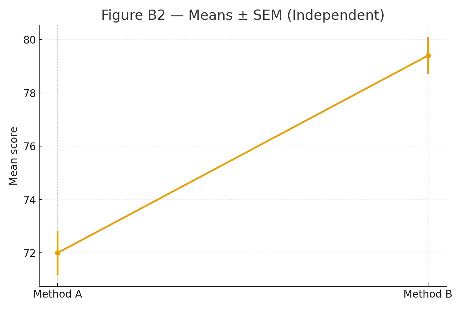
\(\displaystyle \sum A=720 \Rightarrow \bar A=72.0,\qquad \sum B=794 \Rightarrow \bar B=79.4,\qquad \bar A-\bar B=-7.4. \)

Step 2 — Within-Group Variability (sample variances)

  • \(SS_A=60.0 \Rightarrow s_A^2=60/9=6.6667.\)
  • \(SS_B=44.40 \Rightarrow s_B^2=44.40/9=4.9333.\)
Mean exam scores for Methods A and B with standard-error bars.
Figure B2: Group means with SEM error bars.

Step 3 — Pooled Variance & Standard Error (Student’s t)

\(\displaystyle s_p^2=\frac{9(6.6667)+9(4.9333)}{18}=5.8000,\qquad SE=\sqrt{5.8\,(0.1+0.1)}=\sqrt{1.16}=1.0770. \)

Step 4 — Test Statistic, df, p

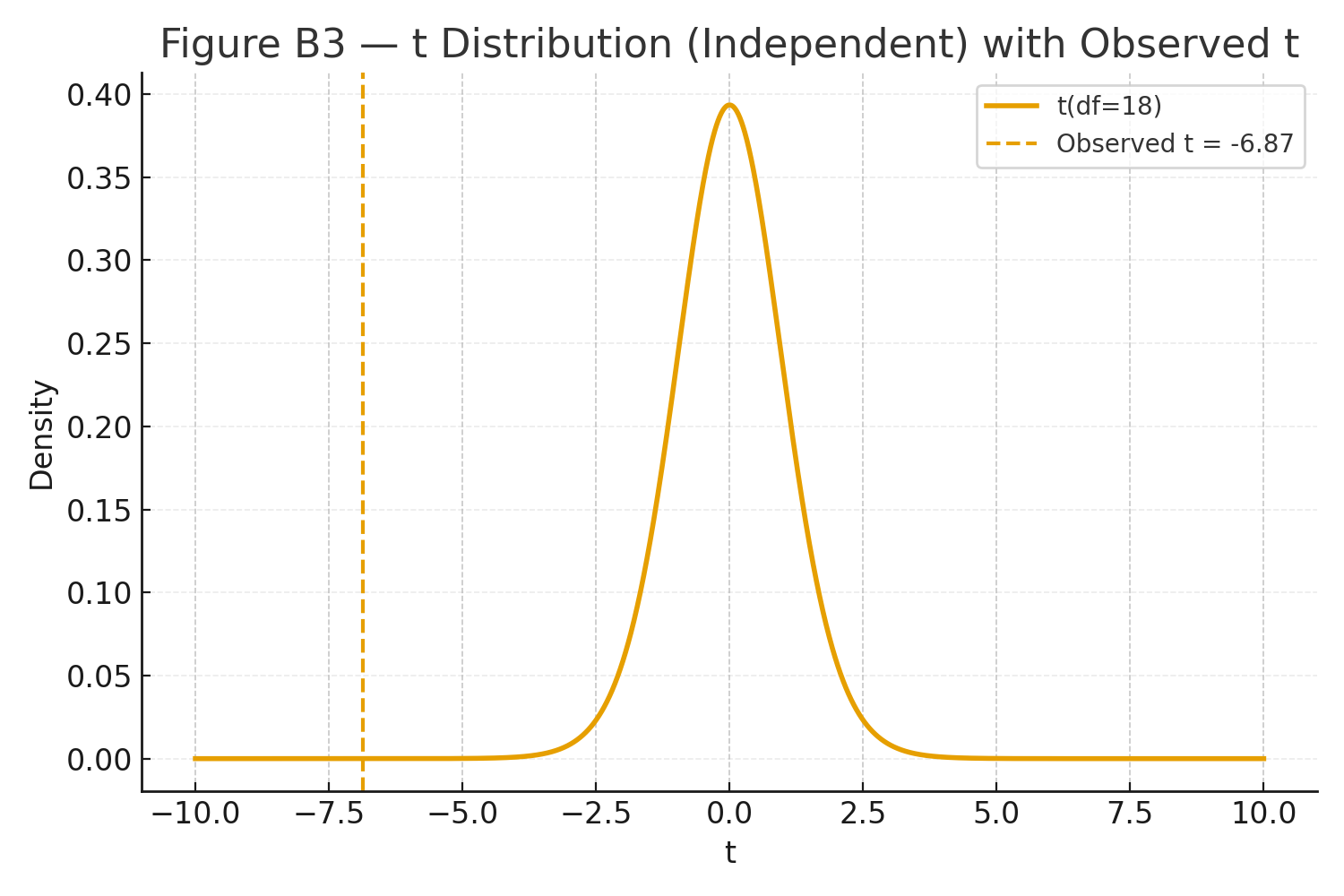
\(\displaystyle t=\frac{-7.4}{1.0770}=-6.872,\qquad df=18,\qquad p\ (\text{two-tailed}) \ll .001. \)

Student t distribution for the independent-samples test with the observed statistic marked in both tails.
Figure B3: t distribution with observed \(t\) marked (two-tailed).

t-Test Summary Table (Independent)

GroupnMeanSDSE(mean)
Method A1072.002.5820.816
Method B1079.402.2220.703
\(\bar A-\bar B\)SE (pooled)tdfp (2-tailed)
-7.401.0770-6.87218< .001

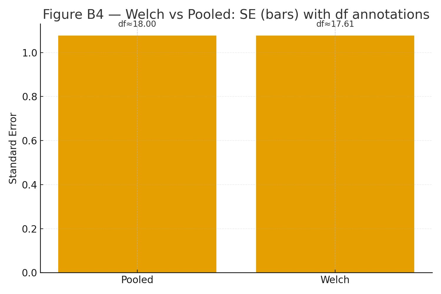
Optional Welch: \(SE_W=\sqrt{0.6667+0.4933}=1.0770,\; df_W\approx 17.61,\; t=-6.872,\; p\ll .001.\)

Comparison of Welch and pooled independent-samples t-test calculations.
Figure B4: Welch vs pooled comparison sketch.

Conclusion (Independent)

Method B yields higher mean scores than Method A (\(t(18)=-6.87,\; p\ll .001\)).


C) Paired-Samples (Dependent) t-Test

Goal. Test whether the mean change (After − Before) differs from zero for the same participants.

Design & Experiment

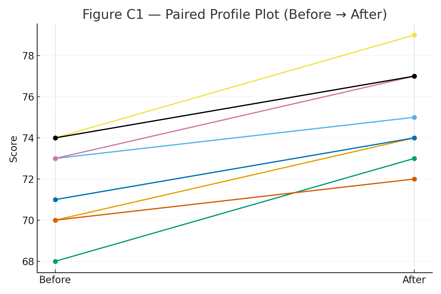
Eight students take an exam before and after a study-skills workshop.

Data

BeforeAfterDifference \(d\) (After − Before)
70744
73752
68735
74795
71743
70722
73774
74773
Before-and-after score profiles for eight students, with lines joining each student’s paired scores.
Figure C1: Paired profile plot (lines per subject) + histogram of differences.

Step 1 — Mean Difference & Variability

\(\sum d = 28 \Rightarrow \bar d = 3.5.\) \(\sum (d-\bar d)^2 = 10 \Rightarrow s_d^2 = 10/7 = 1.4286,\; s_d=1.196.\)

Step 2 — Test Statistic & p-value

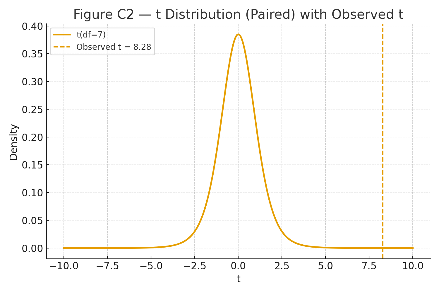
\(\displaystyle SE_{\bar d} = \frac{s_d}{\sqrt{n}}=\frac{1.196}{\sqrt{8}}=0.423,\quad t=\frac{\bar d}{SE_{\bar d}}=\frac{3.5}{0.423}=8.28,\quad df=n-1=7,\quad p\ll .001. \)

Student t distribution with 7 degrees of freedom and the observed paired-test statistic marked.
Figure C2: t curve (df=7) with observed \(t\) marked.

Conclusion (Paired)

Scores were higher after the workshop (\(t(7)=8.28,\; p\ll .001\)); this uncontrolled comparison does not by itself establish that the workshop caused the increase.


Assumptions (checklist)

  • Independent observations (between units; pairing respected for the paired test).
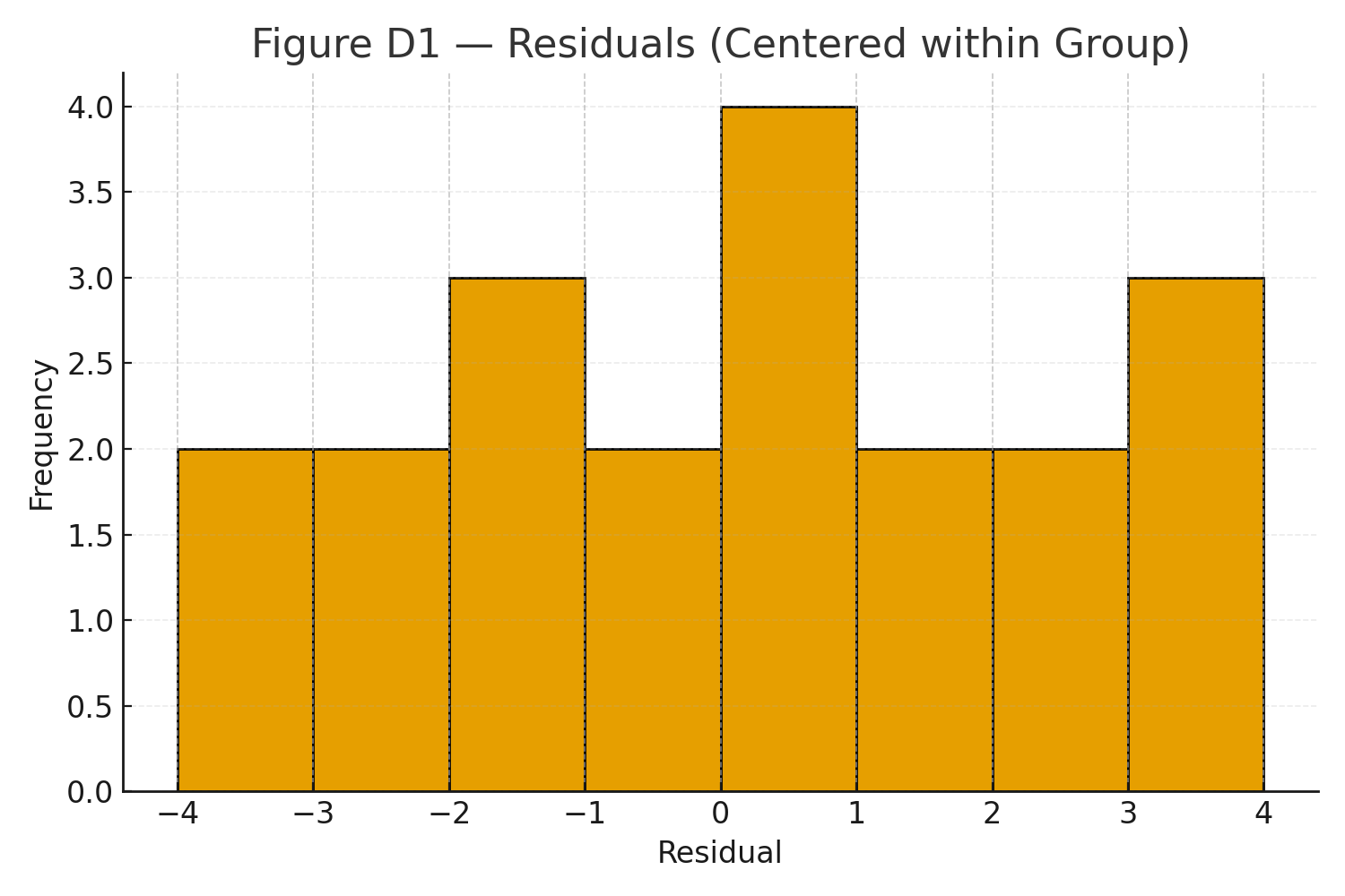
  • Approximately normal residuals (or differences for the paired test).
  • Equal variances only for the pooled independent-samples test; if doubtful, report Welch’s t.
Diagnostic plots illustrating residual distribution and variance checks for t-tests.
Figure D1: QQ plots and Levene/Brown–Forsythe sketch.

Practice self-test quiz

In the space below, please find practice problems and self-test quizzes. For full access, please signup free.
Lesson 5 — Standard Error of the Mean (SEM)

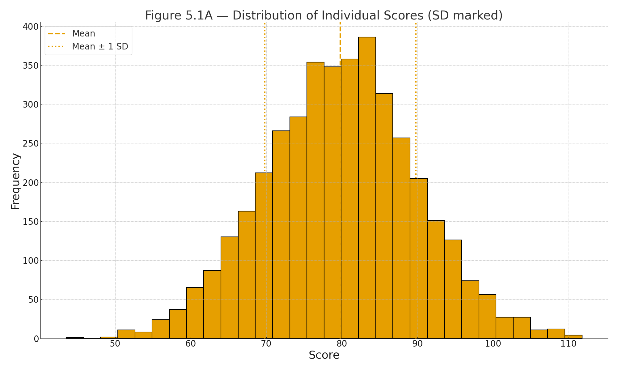
Distribution of individual scores with mean and ±1 SD marked
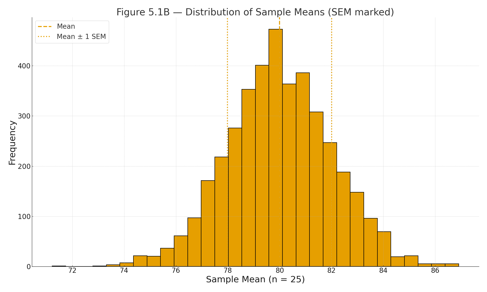
Distribution of sample means (n = 25) with mean and ±1 SEM marked; note the narrower spread
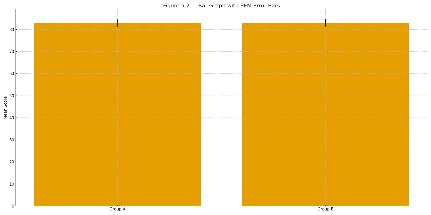
Bar graph of two group means with error bars = SEM

When we take a sample from a population, the sample mean is not always equal to the population mean.
If we took many samples, the sample means would vary.
The Standard Error of the Mean (SEM) tells us how much.

It is the standard deviation of the sampling distribution of the mean.


Formula for the SEM

Symbolic formula:
$$\mathrm{SEM} = \frac{s}{\sqrt{n}}$$

Formula in words:
$$\text{SEM} = \frac{\text{standard deviation}}{\sqrt{\text{number of scores}}}$$

Where:

  • $$s$$ = standard deviation of the sample
  • $$n$$ = number of scores in the sample

Example

A class has test scores with:

  • Mean = 80
  • Standard deviation = 10
  • Sample size = 25

Then:

$$\mathrm{SEM} = \frac{10}{\sqrt{25}} = \frac{10}{5} = 2$$

The SEM is 2.
This means that the mean of repeated samples of 25 students would typically vary about 2 points from the population mean.


Definition

  • Standard Error of the Mean (SEM): the expected variability of a sample mean compared to the true population mean.


Why This Matters

The SEM is crucial for inference.

Visuals

Figure 5.1A — Distribution of individual scores with mean and ±1 SD marked.

Figure 5.1B — Distribution of sample means (n = 25) with mean and ±1 SEM marked; note the narrower spread.

Figure 5.2 — Bar graph of two group means with error bars = SEM.

  • It shows how reliable our sample mean is as an estimate of the population mean.
  • A smaller SEM means a more precise estimate.
  • The SEM appears in formulas for confidence intervals and t-tests.

Practice self-test quiz

In the space below, please find practice problems and self-test quizzes. For full access, please signup free.

Lesson 4 — The Standard Normal Curve

z score
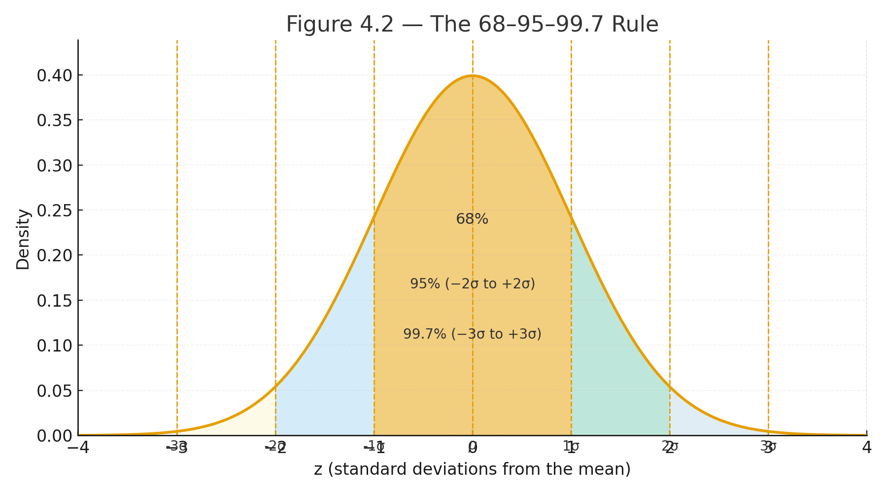
The normal curve. The 68 95 99 rule
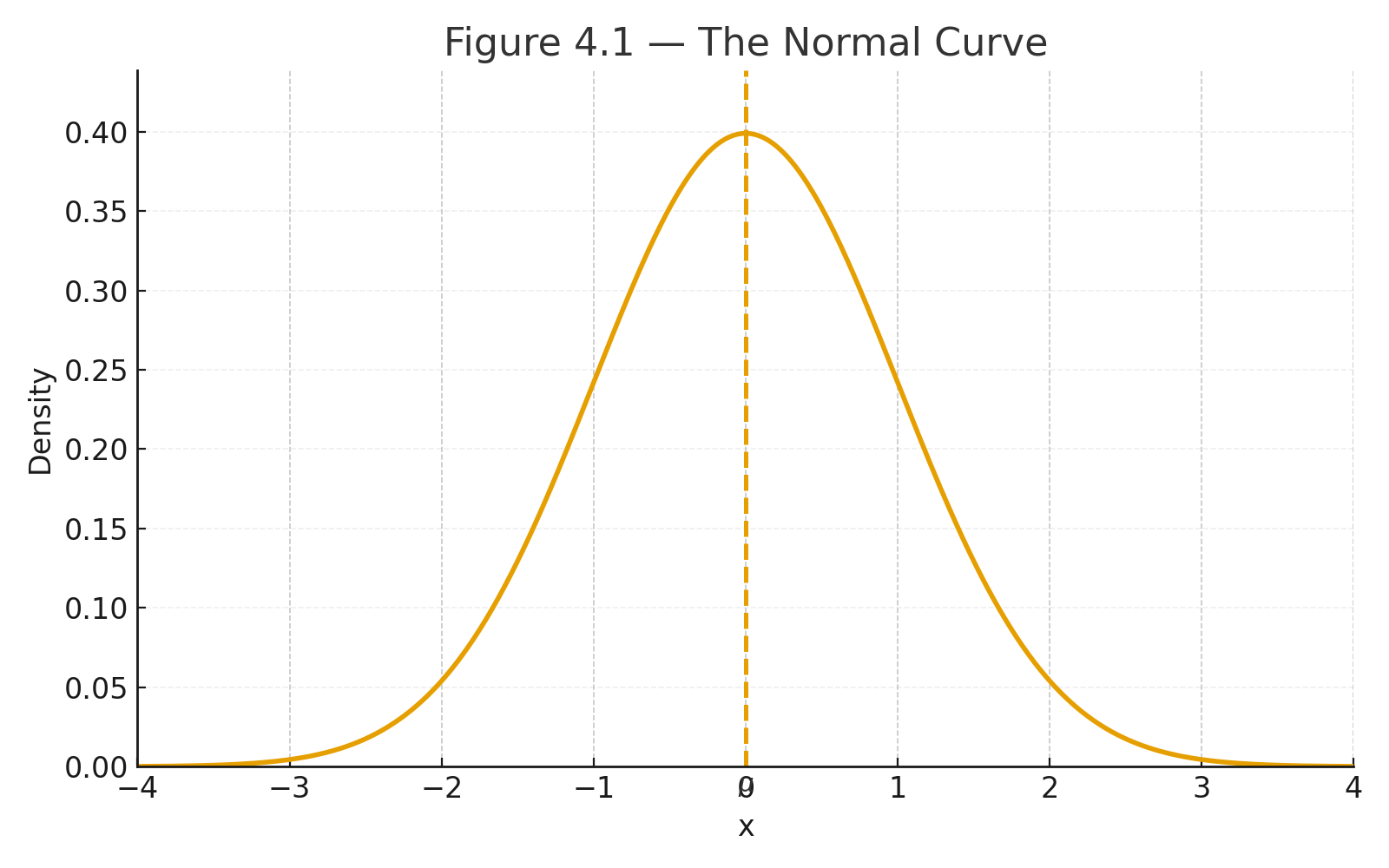
The normal curve

The normal curve (bell curve) is one of the most important shapes in statistics. It appears when many small, independent factors combine: height, test scores, measurement errors.

For a simple, intuitive presentation go to Part 2


Properties of the Normal Curve

  1. Symmetrical around the mean
  2. Unimodal (one peak)
  3. Mean = Median = Mode
  4. The total area under the curve = 1 (or 100%)

Formula for the Normal Distribution

Unless you are in Mathematical Statistics, you will never be asked to reproduce it, or otherwise work with it.

Symbolic formula:
$$f(x) = \frac{1}{\sigma \sqrt{2\pi}} e^{-\frac{(x - \mu)^2}{2\sigma^2}}$$

Formula in words:
$$\text{Probability density} = \frac{1}{\text{standard deviation} \times \sqrt{2\pi}} \times e^{-\frac{(\text{score} - \text{mean})^2}{2 \times (\text{standard deviation})^2}}$$

Where:

  • $$\mu$$ = mean
  • $$\sigma$$ = standard deviation
  • $$x$$ = a value on the curve

Standardization (z-scores)

Symbolic formula:
$$z = \frac{x - \mu}{\sigma}$$

Formula in words:
$$z = \frac{\text{score} - \text{mean}}{\text{standard deviation}}$$

A z-score tells us how many standard deviations a score is above or below the mean.


Key Percentages

Under the normal curve:

  • About 68% of scores are within 1 standard deviation of the mean
  • About 95% are within 2 standard deviations
  • About 99.7% are within 3 standard deviations

This is called the 68–95–99.7 rule.


Example

Suppose test scores are normally distributed with

  • $$\mu = 100$$
  • $$\sigma = 15$$

What is the z-score for a student who scored 115?

$$z = \frac{115 - 100}{15} = \frac{15}{15} = 1$$

This means the student is 1 standard deviation above the mean.


Visuals

Figure 4.1 — The Normal Curve. A bell-shaped curve centered at the mean (μ).

Figure 4.2 — The 68–95–99.7 Rule. A normal curve with shaded regions for ±1σ, ±2σ, ±3σ.

Figure 4.3 — z-Score Example. Normal curve with shaded area to the left of z = 1.0, labeled 0.8413.


Why This Matters

The normal curve is the foundation of inferential statistics.

  • It allows us to compute probabilities.
  • It underlies the t-test, ANOVA, and confidence intervals.
  • By using z-scores, we can compare scores across different tests and distributions.

Practice self-test quiz

In the space below, please find practice problems and self-test quizzes. For full access, please signup free.